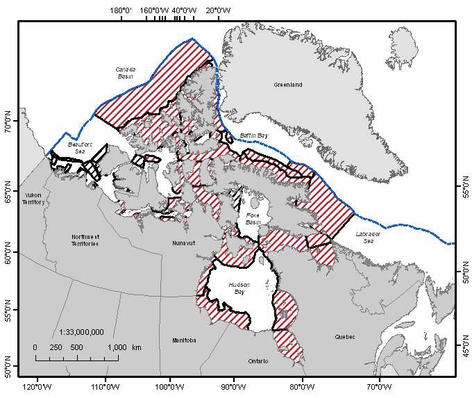
A national Canadian Science Advisory Secretariat (CSAS) science advisory process was held in Winnipeg, Manitoba from June 14-17, 2011 to provide science advice on the identification of Ecologically and Biologically Significant Areas (EBSAs) in the Canadian Arctic based on guidance developed by Fisheries and Oceans Canada. This science advisory process focused on the identification of EBSAs within the following marine biogeographic units: the Hudson Bay Complex, the Arctic Basin, the Western Arctic, the Canadian Arctic Archipelago and the Eastern Arctic. Source: <a href="http://www.dfo-mpo.gc.ca/Library/344747.pdf" target="_blank">Fisheries and Oceans Canada</a> Reference: DFO. 2011. Identification of Ecologically and Biologically Significant Areas (EBSA) in the Canadian Arctic. DFO Can. Sci. Advis. Sec. Sci. Advis. Rep. 2011/055. DFO. 2011. Identification of Ecologically and Biologically Significant Areas (EBSAs) in the Canadian Arctic; June 14-17, 2011. DFO Can. Sci. Advis. Sec. Proceed. Ser. 2011/047.

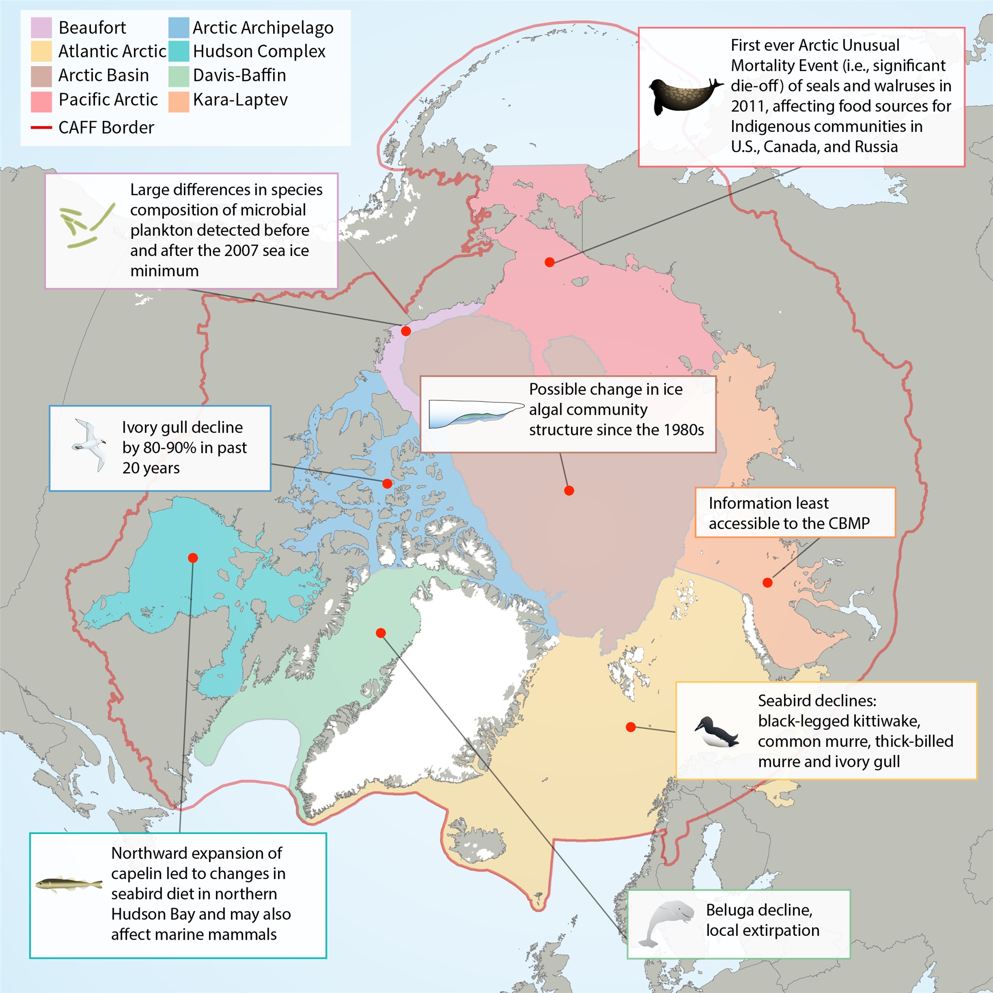
Map of Arctic Marine Areas as defined by the Circumpolar Biodiversity Monitoring Program (CBMP), with one sample finding from each area.

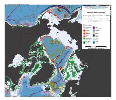
We present the first digital seafloor geomorphic features map (GSFM) of the global ocean. The GSFM includes 131,192 separate polygons in 29 geomorphic feature categories, used here to assess differences between passive and active continental margins as well as between 8 major ocean regions (the Arctic, Indian, North Atlantic, North Pacific, South Atlantic, South Pacific and the Southern Oceans and the Mediterranean and Black Seas). The GSFM provides quantitative assessments of differences between passive and active margins: continental shelf width of passive margins (88 km) is nearly three times that of active margins (31 km); the average width of active slopes (36 km) is less than the average width of passive margin slopes (46 km); active margin slopes contain an area of 3.4 million km2 where the gradient exceeds 5°, compared with 1.3 million km2 on passive margin slopes; the continental rise covers 27 million km2 adjacent to passive margins and less than 2.3 million km2 adjacent to active margins. Examples of specific applications of the GSFM are presented to show that: 1) larger rift valley segments are generally associated with slow-spreading rates and smaller rift valley segments are associated with fast spreading; 2) polar submarine canyons are twice the average size of non-polar canyons and abyssal polar regions exhibit lower seafloor roughness than non-polar regions, expressed as spatially extensive fan, rise and abyssal plain sediment deposits – all of which are attributed here to the effects of continental glaciations; and 3) recognition of seamounts as a separate category of feature from ridges results in a lower estimate of seamount number compared with estimates of previous workers. Reference: Harris PT, Macmillan-Lawler M, Rupp J, Baker EK Geomorphology of the oceans. Marine Geology.

Appendix 9.5 The assignment of liverwort genera of Arctic Russia to families after Konstantinova et al. (2009) and Damsholt (2002)

We present the first digital seafloor geomorphic features map (GSFM) of the global ocean. The GSFM includes 131,192 separate polygons in 29 geomorphic feature categories, used here to assess differences between passive and active continental margins as well as between 8 major ocean regions (the Arctic, Indian, North Atlantic, North Pacific, South Atlantic, South Pacific and the Southern Oceans and the Mediterranean and Black Seas). The GSFM provides quantitative assessments of differences between passive and active margins: continental shelf width of passive margins (88 km) is nearly three times that of active margins (31 km); the average width of active slopes (36 km) is less than the average width of passive margin slopes (46 km); active margin slopes contain an area of 3.4 million km2 where the gradient exceeds 5°, compared with 1.3 million km2 on passive margin slopes; the continental rise covers 27 million km2 adjacent to passive margins and less than 2.3 million km2 adjacent to active margins. Examples of specific applications of the GSFM are presented to show that: 1) larger rift valley segments are generally associated with slow-spreading rates and smaller rift valley segments are associated with fast spreading; 2) polar submarine canyons are twice the average size of non-polar canyons and abyssal polar regions exhibit lower seafloor roughness than non-polar regions, expressed as spatially extensive fan, rise and abyssal plain sediment deposits – all of which are attributed here to the effects of continental glaciations; and 3) recognition of seamounts as a separate category of feature from ridges results in a lower estimate of seamount number compared with estimates of previous workers. Reference: Harris PT, Macmillan-Lawler M, Rupp J, Baker EK Geomorphology of the oceans. Marine Geology.

We present the first digital seafloor geomorphic features map (GSFM) of the global ocean. The GSFM includes 131,192 separate polygons in 29 geomorphic feature categories, used here to assess differences between passive and active continental margins as well as between 8 major ocean regions (the Arctic, Indian, North Atlantic, North Pacific, South Atlantic, South Pacific and the Southern Oceans and the Mediterranean and Black Seas). The GSFM provides quantitative assessments of differences between passive and active margins: continental shelf width of passive margins (88 km) is nearly three times that of active margins (31 km); the average width of active slopes (36 km) is less than the average width of passive margin slopes (46 km); active margin slopes contain an area of 3.4 million km2 where the gradient exceeds 5°, compared with 1.3 million km2 on passive margin slopes; the continental rise covers 27 million km2 adjacent to passive margins and less than 2.3 million km2 adjacent to active margins. Examples of specific applications of the GSFM are presented to show that: 1) larger rift valley segments are generally associated with slow-spreading rates and smaller rift valley segments are associated with fast spreading; 2) polar submarine canyons are twice the average size of non-polar canyons and abyssal polar regions exhibit lower seafloor roughness than non-polar regions, expressed as spatially extensive fan, rise and abyssal plain sediment deposits – all of which are attributed here to the effects of continental glaciations; and 3) recognition of seamounts as a separate category of feature from ridges results in a lower estimate of seamount number compared with estimates of previous workers. Reference: Harris PT, Macmillan-Lawler M, Rupp J, Baker EK Geomorphology of the oceans. Marine Geology.

We present the first digital seafloor geomorphic features map (GSFM) of the global ocean. The GSFM includes 131,192 separate polygons in 29 geomorphic feature categories, used here to assess differences between passive and active continental margins as well as between 8 major ocean regions (the Arctic, Indian, North Atlantic, North Pacific, South Atlantic, South Pacific and the Southern Oceans and the Mediterranean and Black Seas). The GSFM provides quantitative assessments of differences between passive and active margins: continental shelf width of passive margins (88 km) is nearly three times that of active margins (31 km); the average width of active slopes (36 km) is less than the average width of passive margin slopes (46 km); active margin slopes contain an area of 3.4 million km2 where the gradient exceeds 5°, compared with 1.3 million km2 on passive margin slopes; the continental rise covers 27 million km2 adjacent to passive margins and less than 2.3 million km2 adjacent to active margins. Examples of specific applications of the GSFM are presented to show that: 1) larger rift valley segments are generally associated with slow-spreading rates and smaller rift valley segments are associated with fast spreading; 2) polar submarine canyons are twice the average size of non-polar canyons and abyssal polar regions exhibit lower seafloor roughness than non-polar regions, expressed as spatially extensive fan, rise and abyssal plain sediment deposits – all of which are attributed here to the effects of continental glaciations; and 3) recognition of seamounts as a separate category of feature from ridges results in a lower estimate of seamount number compared with estimates of previous workers. Reference: Harris PT, Macmillan-Lawler M, Rupp J, Baker EK Geomorphology of the oceans. Marine Geology.

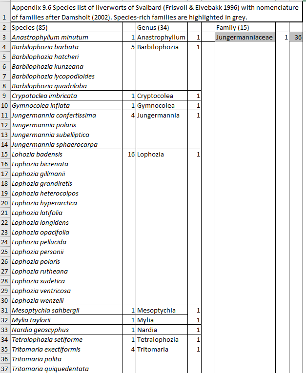
Appendix 9.6 Species list of liverworts of Svalbard (Frisvoll & Elvebakk 1996) with nomenclature of families after Damsholt (2002).

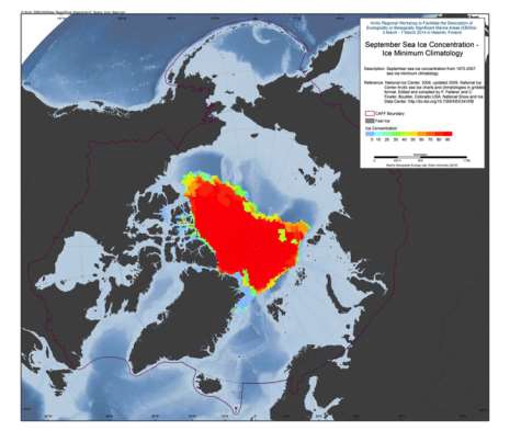
The U.S. National Ice Center (NIC) is an inter-agency sea ice analysis and forecasting center comprised of the Department of Commerce/NOAA, the Department of Defense/U.S. Navy, and the Department of Homeland Security/U.S. Coast Guard components. Since 1972, NIC has produced Arctic and Antarctic sea ice charts. This data set is comprised of Arctic sea ice concentration climatology derived from the NIC weekly or biweekly operational ice-chart time series. The charts used in the climatology are from 1972 through 2007; and the monthly climatology products are median, maximum, minimum, first quartile, and third quartile concentrations, as well as frequency of occurrence of ice at any concentration for the entire period of record as well as for 10-year and 5-year periods. NIC charts are produced through the analyses of available in situ, remote sensing, and model data sources. They are generated primarily for mission planning and safety of navigation. NIC charts generally show more ice than do passive microwave derived sea ice concentrations, particularly in the summer when passive microwave algorithms tend to underestimate ice concentration. The record of sea ice concentration from the NIC series is believed to be more accurate than that from passive microwave sensors, especially from the mid-1990s on (see references at the end of this documentation), but it lacks the consistency of some passive microwave time series. Source: <a href="http://nsidc.org/data/G02172" target="_blank">NSIDC</a> Reference: National Ice Center. 2006, updated 2009. National Ice Center Arctic sea ice charts and climatologies in gridded format. Edited and compiled by F. Fetterer and C. Fowler. Boulder, Colorado USA: National Snow and Ice Data Center. Source: <a href="http://nsidc.org/data/G02172" target="_blank">NSIDC</a>

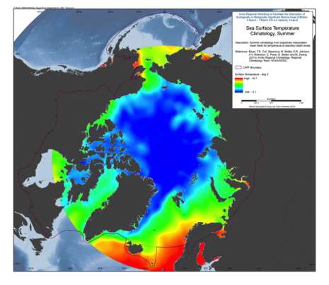
A set of mean fields for temperature and salinity for the Arctic Seas and environs are available for viewing and downloading. Area: The area encompassed is all longitudes from 60°N to 90°N latitudes. Horizontal resolution: Temperature and salinity are available on a 1°x1° and a 1/4°x1/4° latitude/longitude grid. Time resolution: All climatologies for all variables use all available data regardless of year of measurement. Climatologies were calculated for annual (all-data), seasonal, and monthly time periods. Seasons are as follows: Winter (Jan.-Mar.), Spring (Apr.-Jun.), Summer (Jul.-Aug.), Fall (Oct.-Dec.). Vertical resolution: Temperature and salinity are available on 87 standard levels with higher vertical resolution than the World Ocean Atlas 2009 (WOA09), but levels extend from the surface to 4000 m. Units: Temperature units are °C. Salinity is unitless on the Practical Salinity Scale-1978 [PSS]. Data used: All data from the area found in the World Ocean Database (WOD) as of the end of 2011. For a description of this dataset, please see World Ocean Database 2009 Introduction Method: The method followed for calculation of the mean climatological fields is detailed in the following publications: Temperature: Locarnini et al., 2010, Salinity: Antonov et al., 2010. Additional details on the 1/4° climatological calculation are found in Boyer et al., 2005, from: <a href="http://www.nodc.noaa.gov/OC5/regional_climate/arctic/" target="_blank">NOAA</a> Reference: Boyer, T.P., O.K. Baranova, M. Biddle, D.R. Johnson, A.V. Mishonov, C. Paver, D. Seidov and M. Zweng (2012), Arctic Regional Climatology, Regional Climatology Team, NOAA/NODC, source: <a href="www.nodc.noaa.gov/OC5/regional_climate/arctic" target="_blank">NOAA</a>