 CAFF - Arctic Biodiversity Data Service (ABDS)
Type of resources
Available actions
Topics
Keywords
Contact for the resource
Provided by
Years
Formats
Representation types
Update frequencies
status
Service types
Scale
-

We present the first digital seafloor geomorphic features map (GSFM) of the global ocean. The GSFM includes 131,192 separate polygons in 29 geomorphic feature categories, used here to assess differences between passive and active continental margins as well as between 8 major ocean regions (the Arctic, Indian, North Atlantic, North Pacific, South Atlantic, South Pacific and the Southern Oceans and the Mediterranean and Black Seas). The GSFM provides quantitative assessments of differences between passive and active margins: continental shelf width of passive margins (88 km) is nearly three times that of active margins (31 km); the average width of active slopes (36 km) is less than the average width of passive margin slopes (46 km); active margin slopes contain an area of 3.4 million km2 where the gradient exceeds 5°, compared with 1.3 million km2 on passive margin slopes; the continental rise covers 27 million km2 adjacent to passive margins and less than 2.3 million km2 adjacent to active margins. Examples of specific applications of the GSFM are presented to show that: 1) larger rift valley segments are generally associated with slow-spreading rates and smaller rift valley segments are associated with fast spreading; 2) polar submarine canyons are twice the average size of non-polar canyons and abyssal polar regions exhibit lower seafloor roughness than non-polar regions, expressed as spatially extensive fan, rise and abyssal plain sediment deposits – all of which are attributed here to the effects of continental glaciations; and 3) recognition of seamounts as a separate category of feature from ridges results in a lower estimate of seamount number compared with estimates of previous workers. Reference: Harris PT, Macmillan-Lawler M, Rupp J, Baker EK Geomorphology of the oceans. Marine Geology.
-
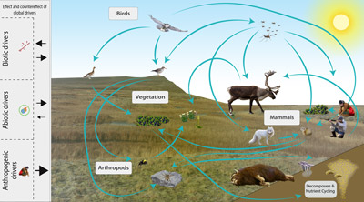
The Arctic terrestrial food web includes the exchange of energy and nutrients. Arrows to and from the driver boxes indicate the relative effect and counter effect of different types of drivers on the ecosystem. STATE OF THE ARCTIC TERRESTRIAL BIODIVERSITY REPORT - Chapter 2 - Page 26- Figure 2.4
-
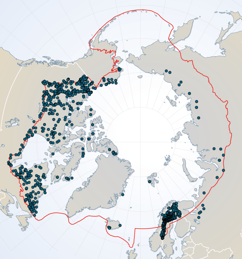
River dataset showing location of study sites in rivers for the Arctic Freshwater Biodiversity Monitoring Plan. Published in the Arctic Freshwater Monitoring Plan Brochure released in 2013 http://www.caff.is/monitoring-series/view_document/277-arctic-freshwater-biodiversity-monitoring-plan-brochure
-
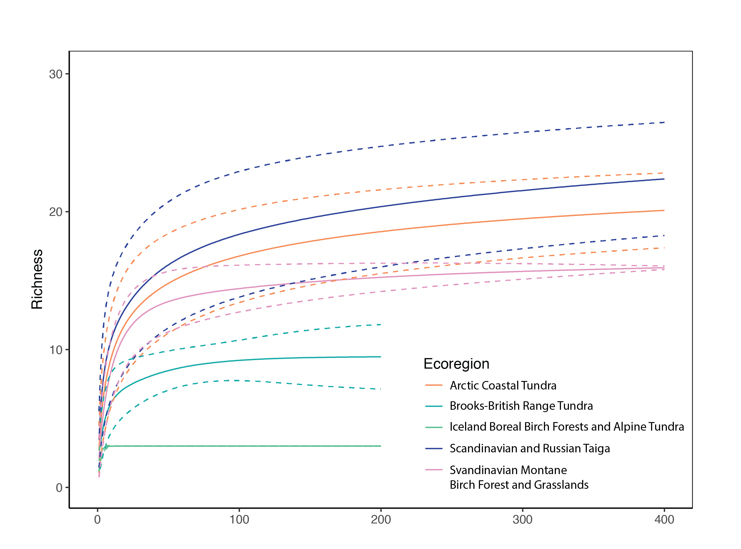
Provides richness estimates and 95% confidence bounds for five ecoregions. State of the Arctic Freshwater Biodiversity Report - Chapter 4 - Page 77 - Figure 4-38
-
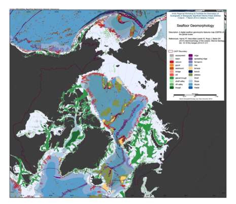
We present the first digital seafloor geomorphic features map (GSFM) of the global ocean. The GSFM includes 131,192 separate polygons in 29 geomorphic feature categories, used here to assess differences between passive and active continental margins as well as between 8 major ocean regions (the Arctic, Indian, North Atlantic, North Pacific, South Atlantic, South Pacific and the Southern Oceans and the Mediterranean and Black Seas). The GSFM provides quantitative assessments of differences between passive and active margins: continental shelf width of passive margins (88 km) is nearly three times that of active margins (31 km); the average width of active slopes (36 km) is less than the average width of passive margin slopes (46 km); active margin slopes contain an area of 3.4 million km2 where the gradient exceeds 5°, compared with 1.3 million km2 on passive margin slopes; the continental rise covers 27 million km2 adjacent to passive margins and less than 2.3 million km2 adjacent to active margins. Examples of specific applications of the GSFM are presented to show that: 1) larger rift valley segments are generally associated with slow-spreading rates and smaller rift valley segments are associated with fast spreading; 2) polar submarine canyons are twice the average size of non-polar canyons and abyssal polar regions exhibit lower seafloor roughness than non-polar regions, expressed as spatially extensive fan, rise and abyssal plain sediment deposits – all of which are attributed here to the effects of continental glaciations; and 3) recognition of seamounts as a separate category of feature from ridges results in a lower estimate of seamount number compared with estimates of previous workers. Reference: Harris PT, Macmillan-Lawler M, Rupp J, Baker EK Geomorphology of the oceans. Marine Geology.
-
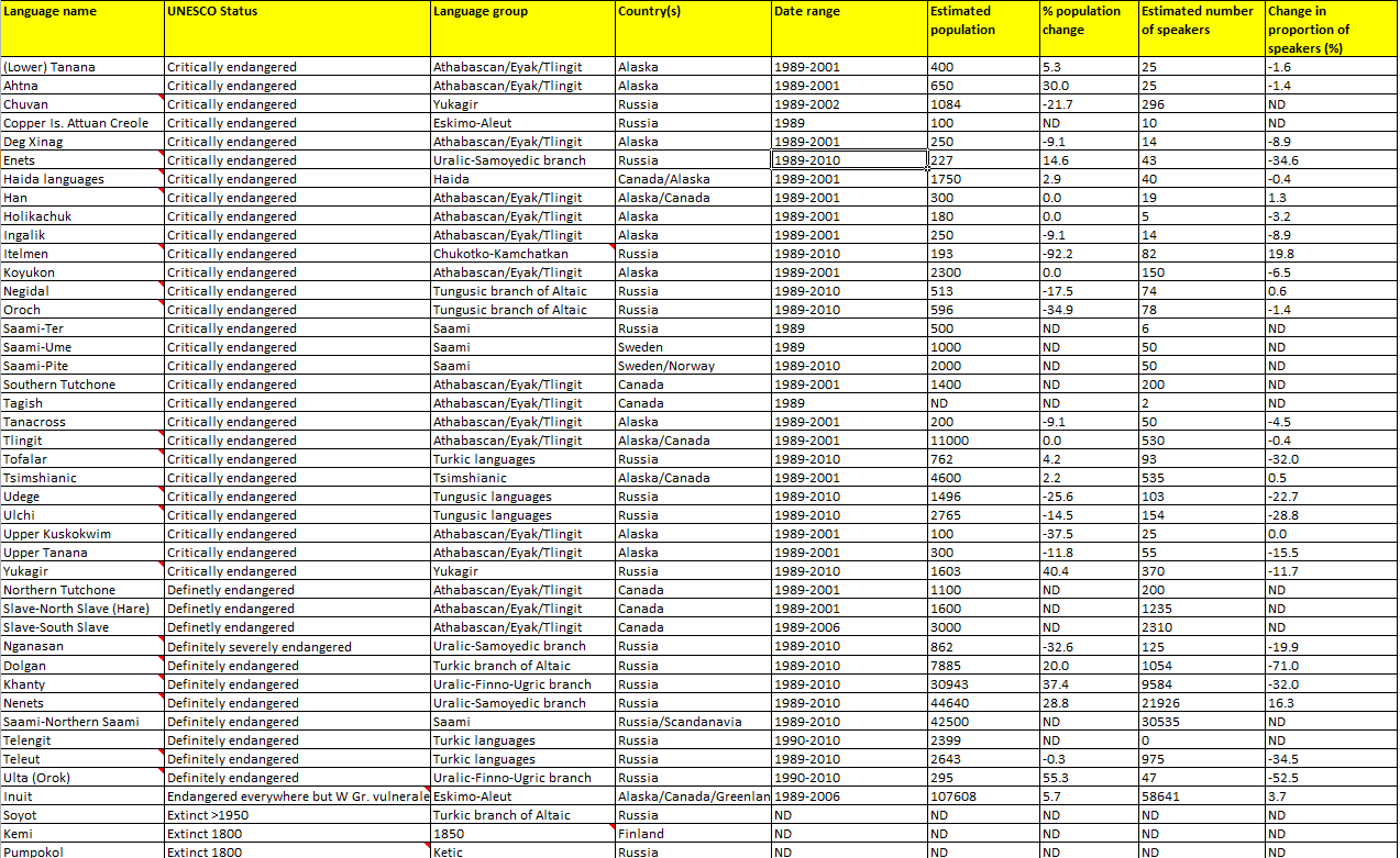
Appendix 20. Arctic indigenous languages status and trends. Data used to compile the information for the table was collected from both census records and academic sources, each of the CAFF countries and indigenous peoples organizations (Permanent Participants to the Arctic Council) where possible also provided statistical information.
-
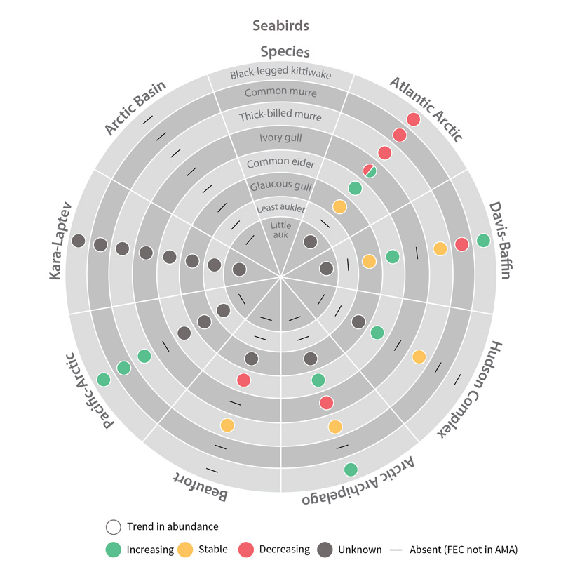
Trends in abundance of seabird Focal Ecosystem Components across each Arctic Marine Area. STATE OF THE ARCTIC MARINE BIODIVERSITY REPORT - Chapter 4 - Page 181 - Figure 4.5
-
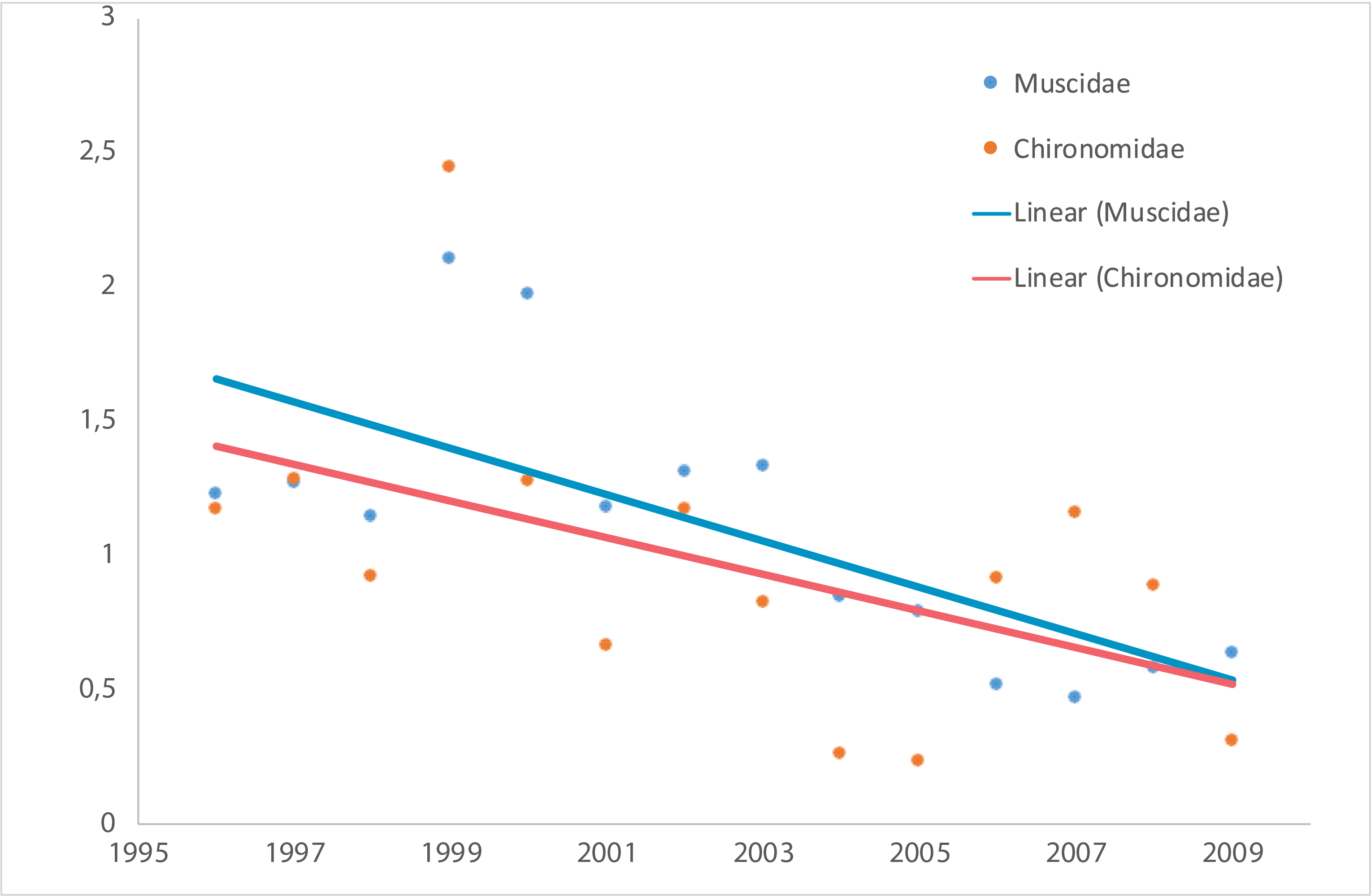
Temporal trends of arthropod abundance, 1996–2009. Estimated by the number of individuals caught per trap per day during the season from four different pitfall trap plots, each consisting of eight (1996–2006) or four (2007–2009) traps. Modified from Høye et al. 2013. STATE OF THE ARCTIC TERRESTRIAL BIODIVERSITY REPORT - Chapter 3 - Page 41 - Figure 3.16
-
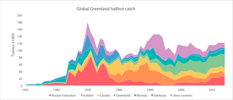
Global catches of Greenland halibut (FAO 2015). STATE OF THE ARCTIC MARINE BIODIVERSITY REPORT - <a href="https://arcticbiodiversity.is/findings/marine-fishes" target="_blank">Chapter 3</a> - Page 121 - Figure 3.4.8
-
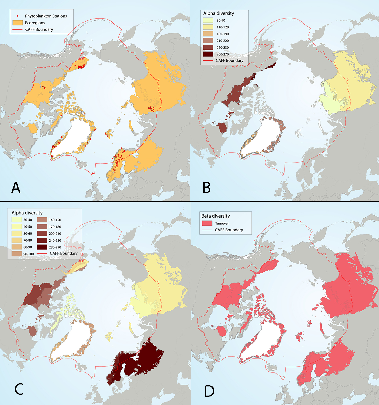
Figure 4 17 Results of circumpolar assessment of lake phytoplankton,(a) the location of phytoplankton stations, underlain by circumpolar ecoregions; (b) ecoregions with many phytoplankton stations, colored on the basis of alpha diversity rarefied to 35 stations; (c) all ecoregions with phytoplankton stations, colored on the basis of alpha diversity rarefied to 10 stations; (d) ecoregions with at least two stations in a hydrobasin, colored on the basis of the dominant component of beta diversity (species turnover, nestedness, approximately equal contribution, or no diversity) when averaged across hydrobasins in each ecoregion. State of the Arctic Freshwater Biodiversity Report - Chapter 4 - Page 56 - Figure 4-17