 CAFF - Arctic Biodiversity Data Service (ABDS)
oceans
Type of resources
Available actions
Topics
Keywords
Contact for the resource
Provided by
Years
Formats
Representation types
Update frequencies
status
Scale
-
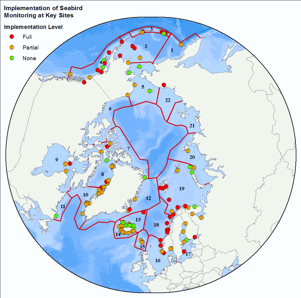
<img width="80px" height="67px" alt="logo" align="left" hspace="10px" src="http://geo.abds.is/geonetwork/srv/eng//resources.get?uuid=7d8986b1-fbd1-4e1a-a7c8-a4cef13e8eca&fname=cbird.png">The Circumpolar Seabird Monitoring Plan is designed to 1) monitor populations of selected Arctic seabird species, in one or more Arctic countries; 2) monitor, as appropriate, survival, diets, breeding phenology, and productivity of seabirds in a manner that allows changes to be detected; 3) provide circumpolar information on the status of seabirds to the management agencies of Arctic countries, in order to broaden their knowledge beyond the boundaries of their country thereby allowing management decisions to be made based on the best available information; 4) inform the public through outreach mechanisms as appropriate; 5) provide information on changes in the marine ecosystem by using seabirds as indicators; and 6) quickly identify areas or issue in the Arctic ecosystem such as declining biodiversity or environmental pressures to target further research and plan management and conservation measures. - <a href="http://caff.is" target="_blank"> Circumpolar Seabird Monitoring plan </a>
-
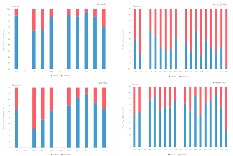
Time series of relative proportions of Arctic and Atlantic Calanus species in Kongsfjorden (top) and Rijpfjorden (bottom) (Source: MOSJ, Norwegian Polar Institute). STATE OF THE ARCTIC MARINE BIODIVERSITY REPORT - <a href="https://arcticbiodiversity.is/findings/plankton" target="_blank">Chapter 3</a> - Page 77 - Figure 3.2.8
-
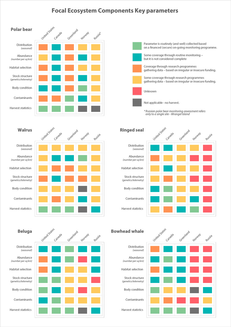
Assessment of monitoring implementation STATE OF THE ARCTIC MARINE BIODIVERSITY REPORT - <a href="https://arcticbiodiversity.is/findings/marine-mammals" target="_blank">Chapter 3</a> - Page 168 - Table 3.6.2
-
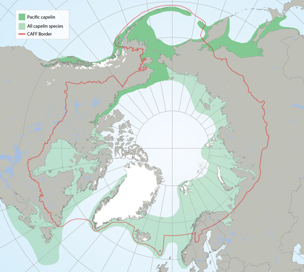
Distributions of all capelin species (light green) and Pacific capelin (Mallotus catervarius; dark green pattern) based on participation in research sampling, examination of museum voucher collections, the literature and molecular genetic analysis (Mecklenburg and Steinke 2015, Mecklenburg et al. 2016). Map shows the maximum distribution observed from point data and includes both common and rare locations STATE OF THE ARCTIC MARINE BIODIVERSITY REPORT - <a href="https://arcticbiodiversity.is/findings/marine-fishes" target="_blank">Chapter 3</a> - Page 117 - Figure 3.4.5
-
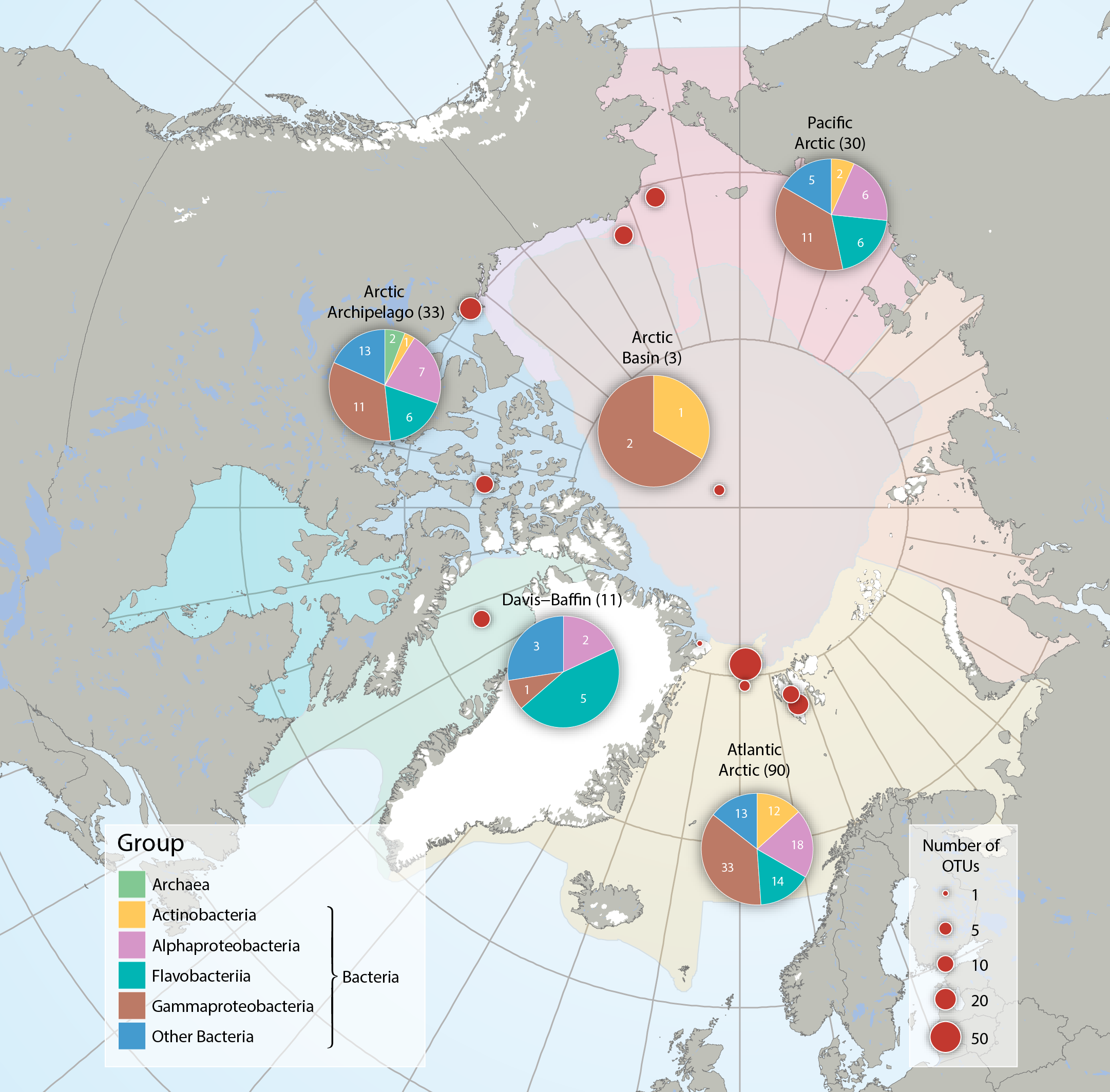
Bacteria and Archaea across five Arctic Marine Areas based on number of operational taxonomic units (OTUs), or molecular species. Composition of microbial groups, with respective numbers of OTUs (pie charts) and number of OTUs at sampling locations (red dots). Data aggregated by the CBMP Sea Ice Biota Expert Network. Data source: National Center for Biotechnology Information’s (NCBI 2017) Nucleotide and PubMed databases. STATE OF THE ARCTIC MARINE BIODIVERSITY REPORT - <a href="https://arcticbiodiversity.is/findings/sea-ice-biota" target="_blank">Chapter 3</a> - Page 38 - Figure 3.1.2 From the report draft: "Synthesis of available data was performed by using searches conducted in the National Center for Biotechnology Information’s “Nucleotide” (http://www.ncbi.nlm.nih.gov/guide/data-software/) and “PubMed” (http://www.ncbi.nlm.nih.gov/pubmed) databases. Aligned DNA sequences were downloaded and clustered into OTUs by maximum likelihood phylogenetic placement."
-
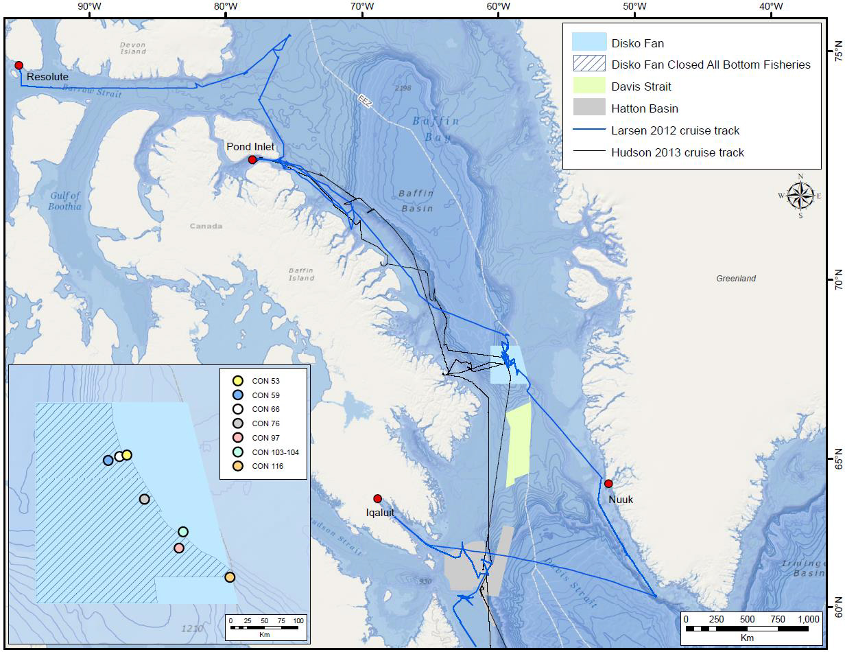
In 2012 and 2013, Fisheries and Oceans Canada conducted benthic imagery surveys in the Davis Strait and Baffin Basin in two areas then closed to bottom fishing, the Hatton Basin Voluntary Closure (now the Hatton Basin Conservation Area) and the Narwhal Closure (now partially in the Disko Fan Conservation Area). The photo transects were established as long-term biodiversity monitoring sites to monitor the impact of human activity, including climate change, on the region’s benthic marine biota in accordance with the protocols of the Circumpolar Biodiversity Monitoring Program established by the Council of Arctic Flora and Fauna. These images were analyzed in a techncial report that summarises the epibenthic megafauna found in seven image transects from the Disko Fan Conservation Area. A total of 480 taxa were found, 280 of which were identified as belonging to one of the following phyla: Annelida, Arthropoda, Brachiopoda, Bryozoa, Chordata, Cnidaria, Echinodermata, Mollusca, Nemertea, and Porifera. The remaining 200 taxa could not be assigned to a phylum and were categorised as Unidentified. Each taxon was identified to the lowest possible taxonomic level, typically class, order, or family. The summaries for each of the taxa include their identification numbers in the World Register of Marine Species and Integrated Taxonomic Information System’s databases, taxonomic hierarchies, images, and written descriptions. The report is intended to provide baseline documentation of the epibenthic megafauna in the Disko Fan Conservation Area, and serve as a taxonomic resource for future image analyses in the Arctic. Baker, E., Beazley, L., McMillan, A., Rowsell, J. and Kenchington, E. 2018. Epibenthic Megafauna of the Disko Fan Conservation Area in the Davis Strait (Eastern Arctic) Identified from In Situ Benthic Image Transects. Can. Tech. Rep. Fish. Aquat. Sci. 3272: vi + 388 p.
-
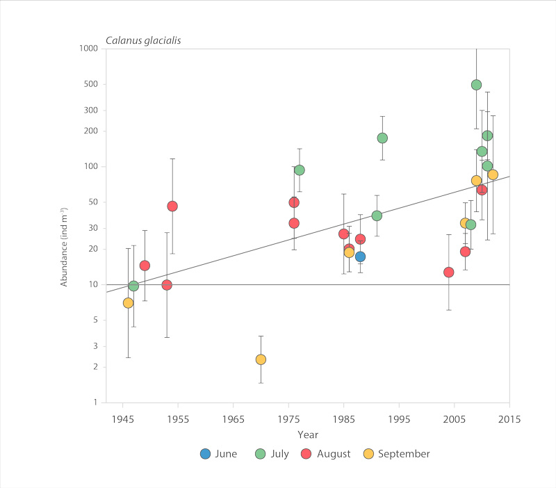
Abundance of the copepod Calanus glacialis in the Chukchi Sea, 1945-2012 (after Ershova et al. 2015b). STATE OF THE ARCTIC MARINE BIODIVERSITY REPORT - <a href="https://arcticbiodiversity.is/findings/plankton" target="_blank">Chapter 3</a> - Page 75 - Figure 3.2.6
-
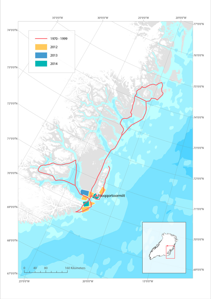
Routes used for hunting polar bear in Ittoqqoortoormiit, East Greenland before 1999 (red line), and in 2012 (yellow), 2013 (blue) and 2014 (green). STATE OF THE ARCTIC MARINE BIODIVERSITY REPORT - <a href="https://arcticbiodiversity.is/findings/marine-mammals" target="_blank">Chapter 3</a> - Page 159 - Box figure 3.6.1
-
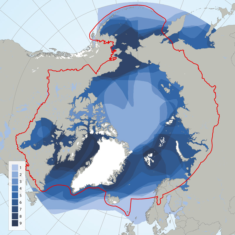
Circumpolar depiction of species richness based on the distributions of the 11 ice-associated Focal Ecosystem Components (according to the distributions reported in IUCN Red List species accounts). A maximum of nine species occur in any one geographic location. The Arctic gateways in both the Atlantic and Pacific regions have the highest species diversity. STATE OF THE ARCTIC MARINE BIODIVERSITY REPORT - <a href="https://arcticbiodiversity.is/findings/marine-mammals" target="_blank">Chapter 3</a> - Page 152 - Figure 3.6.1
-
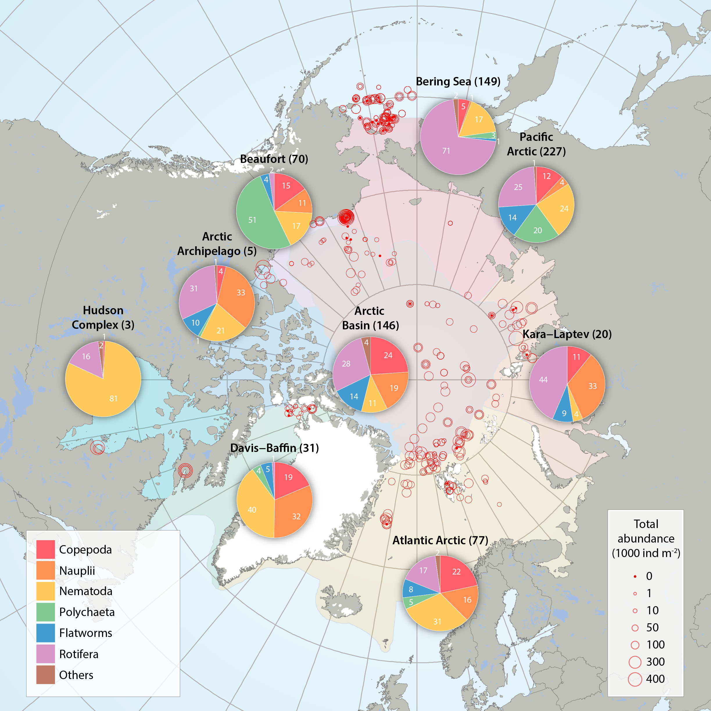
Sea ice meiofauna composition (pie charts) and total abundance (red circles) across the Arctic, compiled by the CBMP Sea Ice Biota Expert Network from 27 studies between 1979 and 2015. Scaled circles show total abundance per individual ice core while pie charts show average relative contribution by taxon per Arctic Marine Area (AMA). Number of ice cores for each AMA is given in parenthesis after region name. Note that studies were conducted at different times of the year, with the majority between March and August (see 3.1 Appendix). The category ‘other’ includes young stages of bristle worms (Polychaeta), mussel shrimps (Ostracoda), forams (Foraminifera), hydroid polyps (Cnidaria), comb jellies (Ctenophora), sea butterflies (Pteropoda), marine mites (Acari) and unidentified organisms. STATE OF THE ARCTIC MARINE BIODIVERSITY REPORT - <a href="https://arcticbiodiversity.is/findings/sea-ice-biota" target="_blank">Chapter 3</a> - Page 40 - Figure 3.1.4 From the report draft: "Here, we synthesized 19 studies across the Arctic conducted between 1979 and 2015, including unpublished sources (B. Bluhm, R. Gradinger, UiT – The Arctic University of Norway; H. Hop, Norwegian Polar Institute; K. Iken, University of Alaska Fairbanks). These studies sampled landfast sea ice and offshore pack ice, both first- and multiyear ice (Appendix 3.1). Meiofauna abundances reported in individual data sources were converted to individuals m-2 of sea ice assuming that ice density was 95% of that in melted ice. Due to the low taxonomic resolution in the reviewed studies, ice meiofauna were grouped into: Copepoda, nauplii (for copepods as well as other taxa with naupliar stages), Nematoda, Polychaeta (mostly juveniles, but also trochophores), flatworms (Acoelomorpha and Platyhelminthes; these phyla have mostly been reported as one category), Rotifera, and others (which include meroplanktonic larvae other than Polychaeta, Ostracoda, Foraminifera, Cnidaria, Ctenophora, Pteropoda, Acari, and unidentified organisms). Percentage of total abundance for each group was calculated for each ice core, and these percentages were used for regional averages. Maximum available ice core length was used in data analysis, but 50% of these ice cores included only the bottom 10 cm of the ice, 12% the bottom 5 cm, 10% the bottom 2 cm, and 11% the entire ice-thickness. Data from 617 cores were used."