 CAFF - Arctic Biodiversity Data Service (ABDS)
Type of resources
Available actions
Topics
Keywords
Contact for the resource
Provided by
Years
Formats
Representation types
Update frequencies
status
Service types
Scale
-
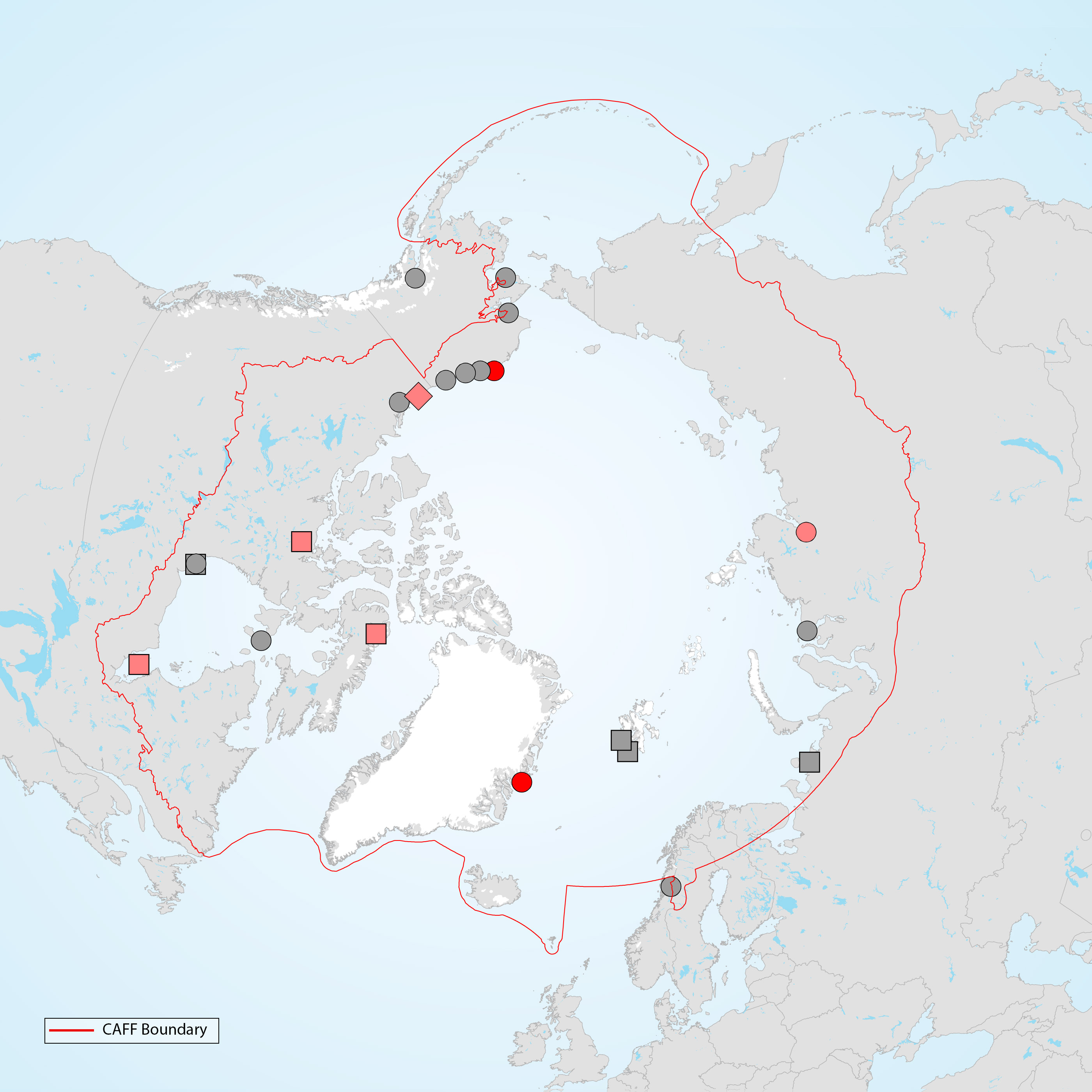
Study sites across the Arctic where phenological mismatches between timing of reproduction and peak abundance in food have been studied for terrestrial bird species. Grey symbols show study sites where this phenomenon has been studied for <10 years, light red symbols show sites with >10 years of data but no strong evidence of an increasing mismatch, and dark red symbols indicate sites with >10 years of data and strong evidence of an increasing mismatch. Circles indicate studies of shorebirds, squares for waterfowl and diamonds(triancle) for both shorebirds and passerines. Graphic: Thomas Lameris, adapted from Zhemchuzhnikov (submitted). STATE OF THE ARCTIC TERRESTRIAL BIODIVERSITY REPORT - Chapter 3 - Page 65 - Figure Box 3.3
-
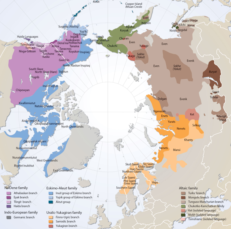
The North is inhabited by an array of peoples with different cultures and language groupings. For this report, information was compiled on 89 northern languages which accounts for a little more than 1% of the worlds living languages3. These can be grouped into six distinct language families plus three isolated languages presently unconnected to any other language grouping (Fig. 20.1). Conservation of Arctic Flora and Fauna, CAFF 2013 - Akureyri . Arctic Biodiversity Assessment. Status and Trends in Arctic biodiversity. - Linguistic Diversity (Chapter 20) page 656
-
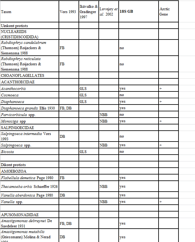
Appendix 11. Taxa of hetorotrophic protists reported from Foxe Basin, Canada (FB), Disko Bay, W Greenland (DB; Vors 1993), the Greenland Sea (GLS; Ikävalko & Gradinger 1997) and Northern Baffin Bay, Canada (NBB; Lovejoy et al. 2002).
-
The Seabird Information Network (SIN) developed by the Circumpolar Seabird expert group (<a href="http://caff.is/seabirds-cbird" target="_blank">CBird</a>) of the Conservation of Arctic Flora and Fauna (<a href="http://caff.is" target="_blank">CAFF</a>) working group of the Arctic Council focuses on the development of a data entry and analysis portal system allowing for circumpolar seabird colony information to be contributed, mapped, and shared by scientists and monitoring programs around the Arctic. - <a href="http://axiom.seabirds.net/maps/js/seabirds.php?app=circumpolar#z=2&ll=NaN,0.00000" target="_blank"> Circumpolar Seabird portal</a>
-
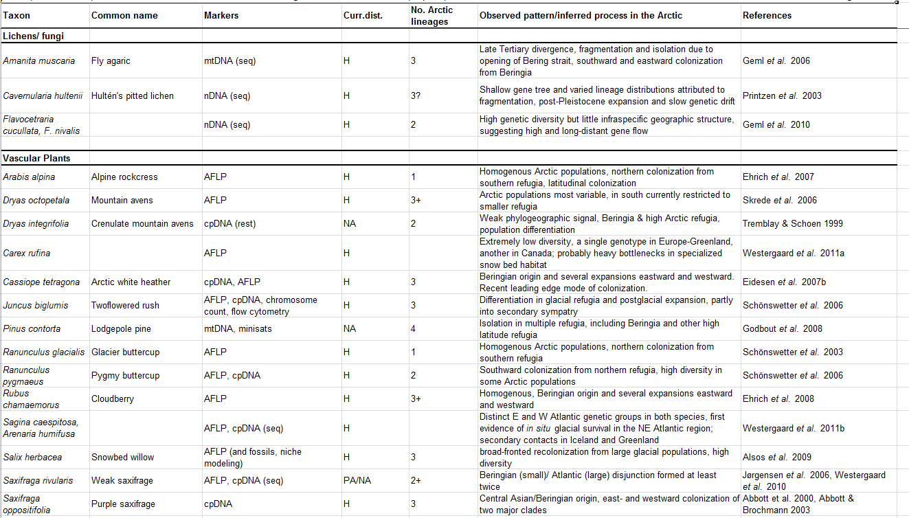
Appendix 17.3. Phylogeographic and population genetics studies of selected Arctic species.
-
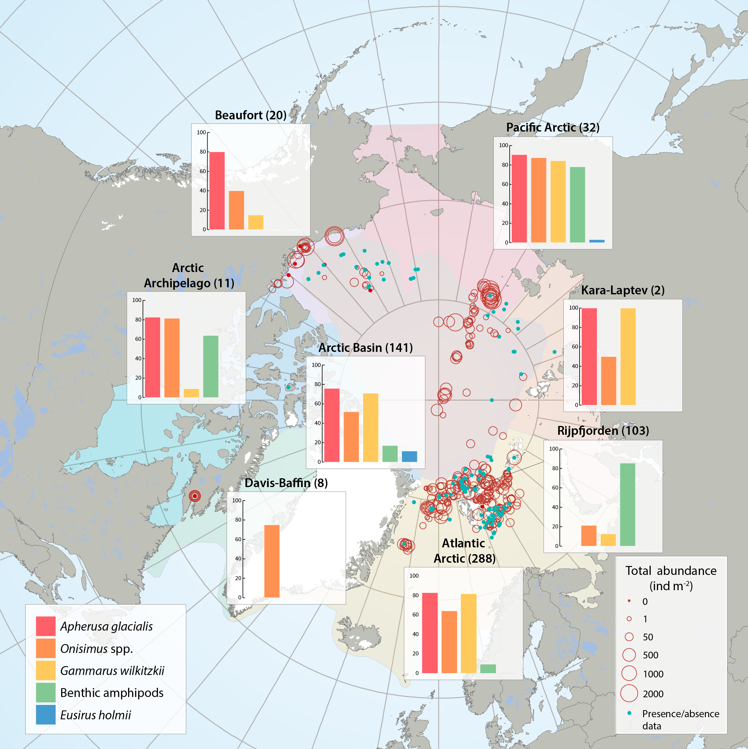
Sea ice amphipod (macrofauna) distribution and abundance across the Arctic aggregated from 47 sources between 1977 and 2012 by the CBMP Sea Ice Biota Expert Network. Bar graphs illustrate the frequency of occurrence (%) of amphipods in samples that contained at least one ice-associated amphipod. Red circles illustrate the total abundances of all ice-associated amphipods in quantitative samples (individuals m-2) at locations of sampling for each Arctic Marine Area (AMA). Number of sampling efforts for each region is given in parenthesis after region name. Blue dots represent samples where only presence/ absence data were available and where amphipods were present. STATE OF THE ARCTIC MARINE BIODIVERSITY REPORT - <a href="https://arcticbiodiversity.is/findings/sea-ice-biota" target="_blank">Chapter 3</a> - Page 44 - Figure 3.1.6 From the report draft: "This summary includes 47 data sources of under-ice amphipods published between 1977 and 2012. When available, we collected information on abundance or density (ind. m-2, or ind. m-3 that were converted to ind. m-2) and biomass (g m-2, wet weight). If abundance or biomass data were not available, we examined presence/relative abundance information. Frequency of occurrence was calculated for regions across the Arctic using integrated data for all available years."
-
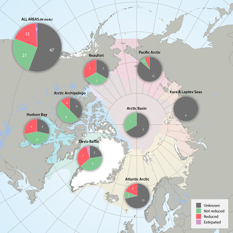
Status of marine mammal Focal Ecosystem Component stocks by Arctic Marine Area. STATE OF THE ARCTIC MARINE BIODIVERSITY REPORT - <a href="https://arcticbiodiversity.is/findings/marine-mammals" target="_blank">Chapter 3</a> - Page 157 - Figure 3.6.3
-
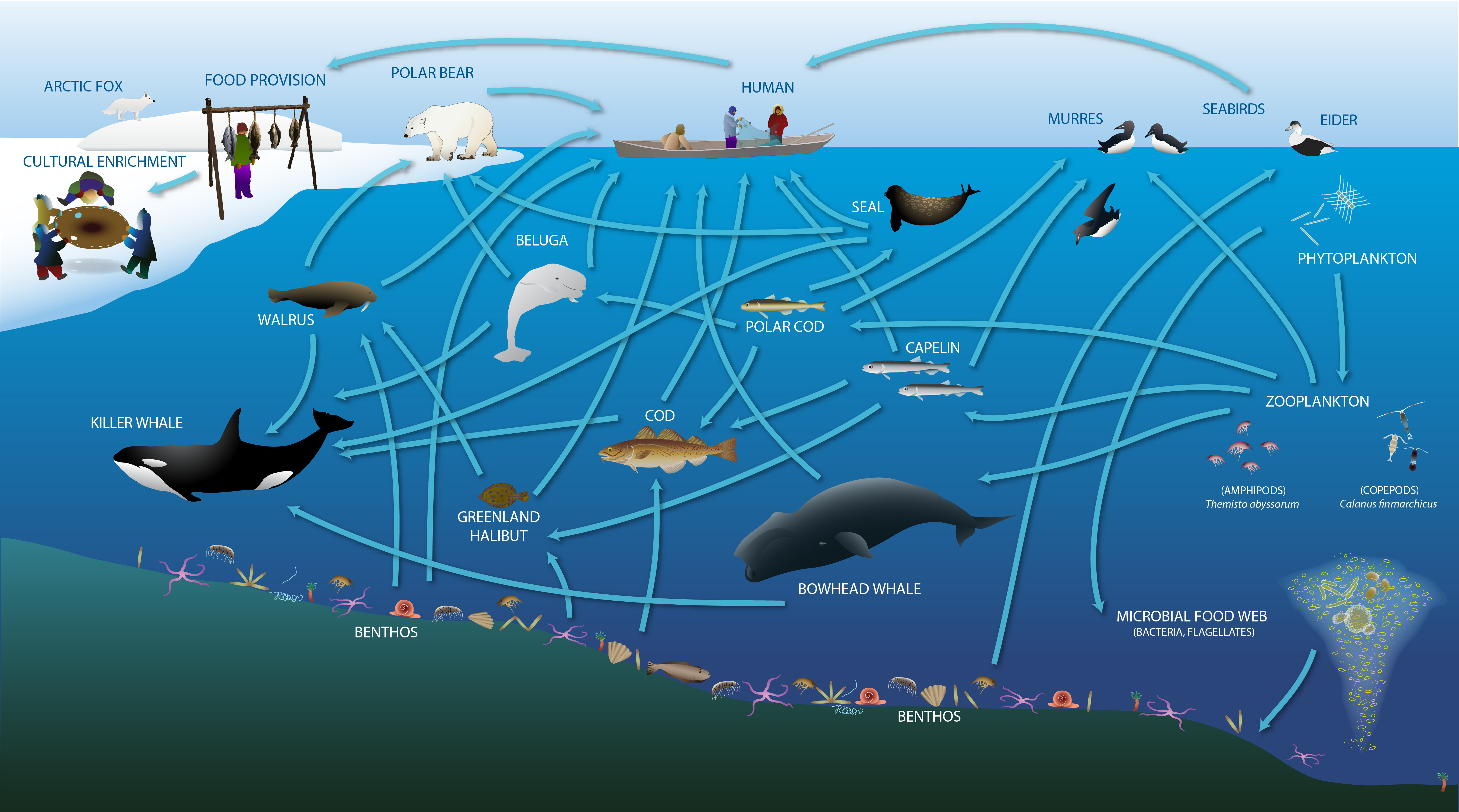
Changes expected or underway in the of energy flow in the High Arctic marine environment STATE OF THE ARCTIC MARINE BIODIVERSITY REPORT - <a href="https://arcticbiodiversity.is/marine" target="_blank">Chapter 2</a> - Page 23 - Figure 2.2b
-
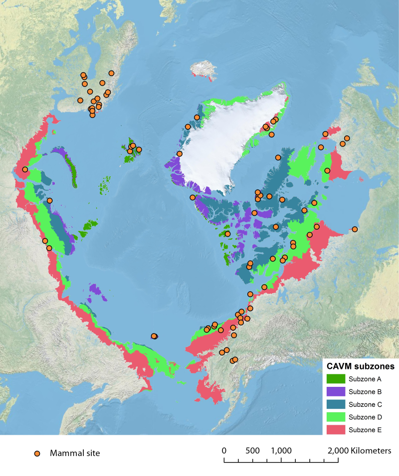
Location of long-term mammal monitoring sites and programs. Comes from the Arctic Terrestrial Biodiversity Monitoring Plan is developed to improve the collective ability of Arctic traditional knowledge holders, northern communities and scientists to detect, understand and report on long-term change in Arctic terrestrial ecosystems and biodiversity..
-
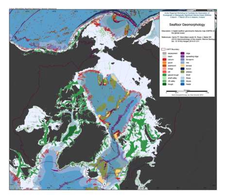
We present the first digital seafloor geomorphic features map (GSFM) of the global ocean. The GSFM includes 131,192 separate polygons in 29 geomorphic feature categories, used here to assess differences between passive and active continental margins as well as between 8 major ocean regions (the Arctic, Indian, North Atlantic, North Pacific, South Atlantic, South Pacific and the Southern Oceans and the Mediterranean and Black Seas). The GSFM provides quantitative assessments of differences between passive and active margins: continental shelf width of passive margins (88 km) is nearly three times that of active margins (31 km); the average width of active slopes (36 km) is less than the average width of passive margin slopes (46 km); active margin slopes contain an area of 3.4 million km2 where the gradient exceeds 5°, compared with 1.3 million km2 on passive margin slopes; the continental rise covers 27 million km2 adjacent to passive margins and less than 2.3 million km2 adjacent to active margins. Examples of specific applications of the GSFM are presented to show that: 1) larger rift valley segments are generally associated with slow-spreading rates and smaller rift valley segments are associated with fast spreading; 2) polar submarine canyons are twice the average size of non-polar canyons and abyssal polar regions exhibit lower seafloor roughness than non-polar regions, expressed as spatially extensive fan, rise and abyssal plain sediment deposits – all of which are attributed here to the effects of continental glaciations; and 3) recognition of seamounts as a separate category of feature from ridges results in a lower estimate of seamount number compared with estimates of previous workers. Reference: Harris PT, Macmillan-Lawler M, Rupp J, Baker EK Geomorphology of the oceans. Marine Geology.