 CAFF - Arctic Biodiversity Data Service (ABDS)
Land cover
Type of resources
Available actions
Topics
Keywords
Contact for the resource
Provided by
Years
Formats
Representation types
Update frequencies
status
-
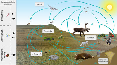
The Arctic terrestrial food web includes the exchange of energy and nutrients. Arrows to and from the driver boxes indicate the relative effect and counter effect of different types of drivers on the ecosystem. STATE OF THE ARCTIC TERRESTRIAL BIODIVERSITY REPORT - Chapter 2 - Page 26- Figure 2.4
-
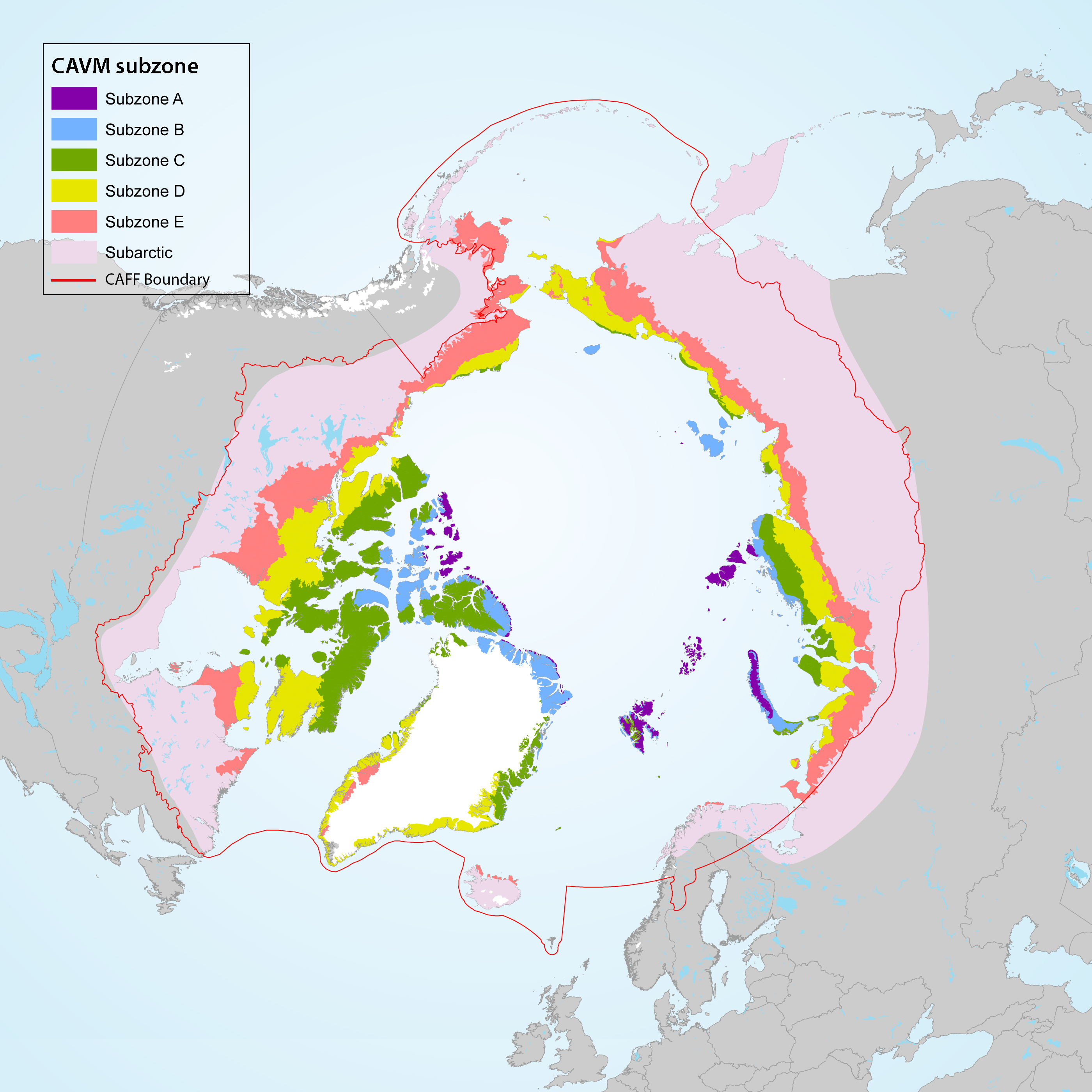
Geographic area covered by the Arctic Biodiversity Assessment and the CBMP–Terrestrial Plan. Subzones A to E are depicted as defined in the Circumpolar Arctic Vegetation Map (CAVM Team 2003). Subzones A, B and C are the high Arctic while subzones D and E are the low Arctic. Definition of high Arctic, low Arctic, and sub-Arctic follow Hohn & Jaakkola 2010. STATE OF THE ARCTIC TERRESTRIAL BIODIVERSITY REPORT - Chapter 1 - Page 14 - Figure 1.2
-
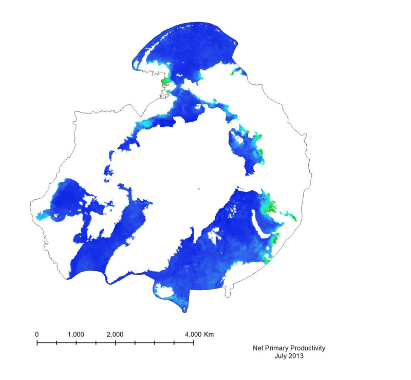
Marine primary productivity is not available from the NASA Ocean Color website. Currently the best product available for marine primary productivity is available through Oregon State University’s Ocean Productivity Project. A monthly global Net Primary Productivity product at 9 km spatial resolution has been selected for this analysis. The algorithm used to create the primary productivity is a Vertically Generalized Production Model (VGPM) created by Behrenfeld and Falkowski (1997). It is a “chlorophyll-based” model that estimates net primary production from chlorophyll using a temperature-dependent description of chlorophyll photosynthetic efficiency (O’Malley 2010). Inputs to the function are chlorophyll, available light, and photosynthetic efficiency.
-
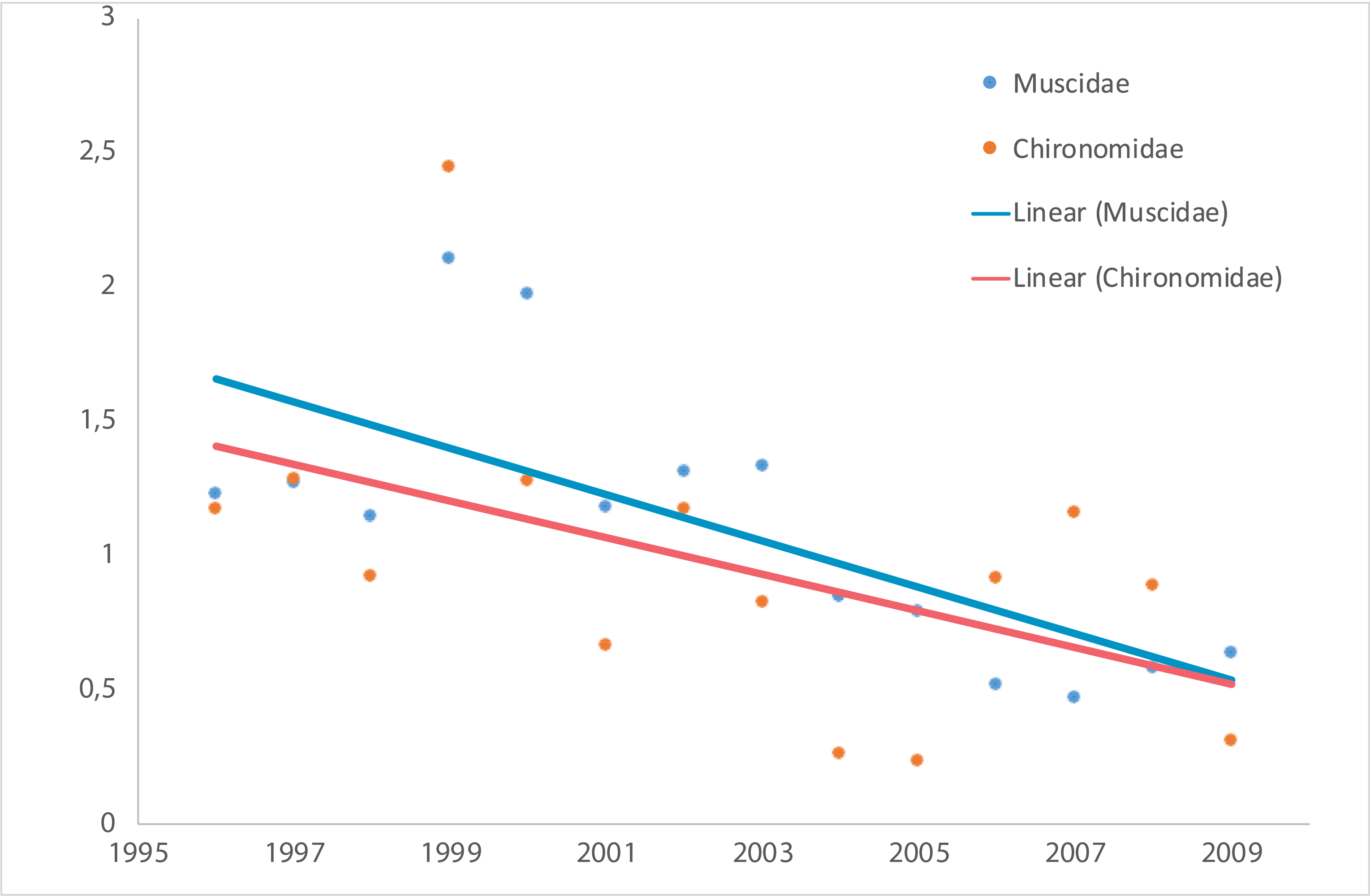
Temporal trends of arthropod abundance, 1996–2009. Estimated by the number of individuals caught per trap per day during the season from four different pitfall trap plots, each consisting of eight (1996–2006) or four (2007–2009) traps. Modified from Høye et al. 2013. STATE OF THE ARCTIC TERRESTRIAL BIODIVERSITY REPORT - Chapter 3 - Page 41 - Figure 3.16
-
Change in plant phenology over time based on published studies, ranging from 9 to 21 years of duration. The bars show the proportion of observations where timing of phenological events advanced (earlier) was stable or were delayed (later) over time. The darker portions of each bar represent visible decrease, stable state, or increase results, and lighter portions represent marginally significant change. The numbers above each bar indicate the number of observations in that group. Figure from Bjorkman et al. 2020. STATE OF THE ARCTIC TERRESTRIAL BIODIVERSITY REPORT - Chapter 3 - Page 31- Figure 3.3
-
Temporal trends of arthropod abundance for three habitat types at Zackenberg Research Station, Greenland, 1996–2016. Data are grouped as the FEC ‘arthropod prey for vertebrates’ and separated by habitat type. Solid lines indicate significant regression lines at the p<0.05. Modified from Gillespie et al. 2020a. STATE OF THE ARCTIC TERRESTRIAL BIODIVERSITY REPORT - Chapter 3 - Page 39 - Figure 3.9
-
Many population counts of gregarious migrant species, such as waders and geese, take place along the flyways and at wintering grounds outside the Arctic which stresses the importance of continued development of movement ecology studies. Monitoring of FEC attributes related to breeding success and links to environmental drivers within the Arctic takes place in a wide network of research sites across the Arctic, although with low coverage of the high Arctic zone (Figure 3-25) STATE OF THE ARCTIC TERRESTRIAL BIODIVERSITY REPORT - Chapter 3 - Page 58 - Figure 3.25
-
Trends in Arctic terrestrial bird population abundance for four taxonomic groupings in four global flyways. Data are presented as total number of taxa (species, subspecies). Modified from Smith et al. 2020. These broad patterns were generally consistent across flyways, with some exceptions. Fewer waterfowl populations increased in the Central Asian and East Asian–Australasian Flyways. The largest proportion of declining species was among the waders in all but the Central Asian Flyway where the trends of a large majority of waders are unknown. Although declines were more prevalent among waders than other taxonomic groups in both the African–Eurasian and Americas Flyways, the former had a substantially larger number of stable and increasing species than the latter (Figure 3-23). STATE OF THE ARCTIC TERRESTRIAL BIODIVERSITY REPORT - Chapter 3 - Page 55 - Figure 3.23
-
Population trends for springtails in Empetrum nigrum plant community in Kobbefjord, Greenland, 2007–2017. (a) mean population abundance of total Collembola in individuals per square metre, (b) mean number of species per sample, and (c) Shannon-Wiener diversity index per sample. Vertical error bars are standard errors of the mean. Solid lines indicate significant regression lines. Modified from Gillespie et al. 2020a. STATE OF THE ARCTIC TERRESTRIAL BIODIVERSITY REPORT - Chapter 3 - Page 40 - Figure 3.13
-
Population estimates and trends for Rangifer populations of the migratory tundra, Arctic island, mountain, and forest ecotypes where their circumpolar distribution intersects the CAFF boundary. Population trends (Increasing, Stable, Decreasing, or Unknown) are indicated by shading. Data sources for each population are indicated as footnotes. STATE OF THE ARCTIC TERRESTRIAL BIODIVERSITY REPORT - Chapter 3 - Page 70 - Table 3.4