 CAFF - Arctic Biodiversity Data Service (ABDS)
Type of resources
Available actions
Topics
Keywords
Contact for the resource
Provided by
Years
Formats
Representation types
Update frequencies
status
Service types
Scale
-
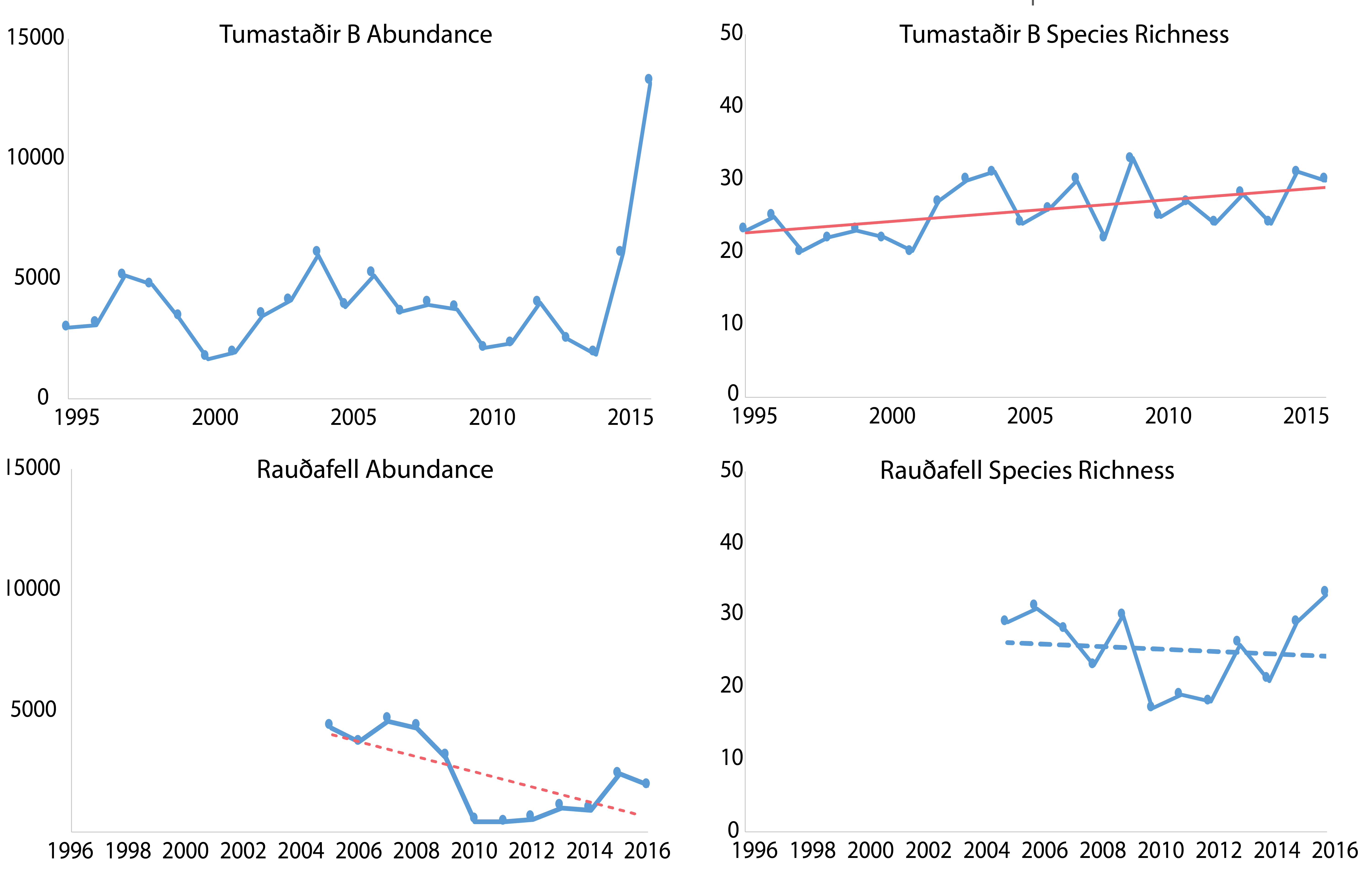
Trends in total abundance of moths and species richness, from two locations in Iceland, 1995–2016. Trends differ between locations. The solid and dashed straight lines represent linear regression lines which are significant or non-significant, respectively. Modified from Gillespie et al. 2020a. STATE OF THE ARCTIC TERRESTRIAL BIODIVERSITY REPORT - Chapter 3 - Page 41 - Figure 3.14
-
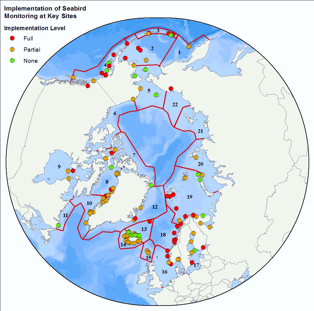
<img width="80px" height="67px" alt="logo" align="left" hspace="10px" src="http://geo.abds.is/geonetwork/srv/eng//resources.get?uuid=7d8986b1-fbd1-4e1a-a7c8-a4cef13e8eca&fname=cbird.png">The Circumpolar Seabird Monitoring Plan is designed to 1) monitor populations of selected Arctic seabird species, in one or more Arctic countries; 2) monitor, as appropriate, survival, diets, breeding phenology, and productivity of seabirds in a manner that allows changes to be detected; 3) provide circumpolar information on the status of seabirds to the management agencies of Arctic countries, in order to broaden their knowledge beyond the boundaries of their country thereby allowing management decisions to be made based on the best available information; 4) inform the public through outreach mechanisms as appropriate; 5) provide information on changes in the marine ecosystem by using seabirds as indicators; and 6) quickly identify areas or issue in the Arctic ecosystem such as declining biodiversity or environmental pressures to target further research and plan management and conservation measures. - <a href="http://caff.is" target="_blank"> Circumpolar Seabird Monitoring plan </a>
-
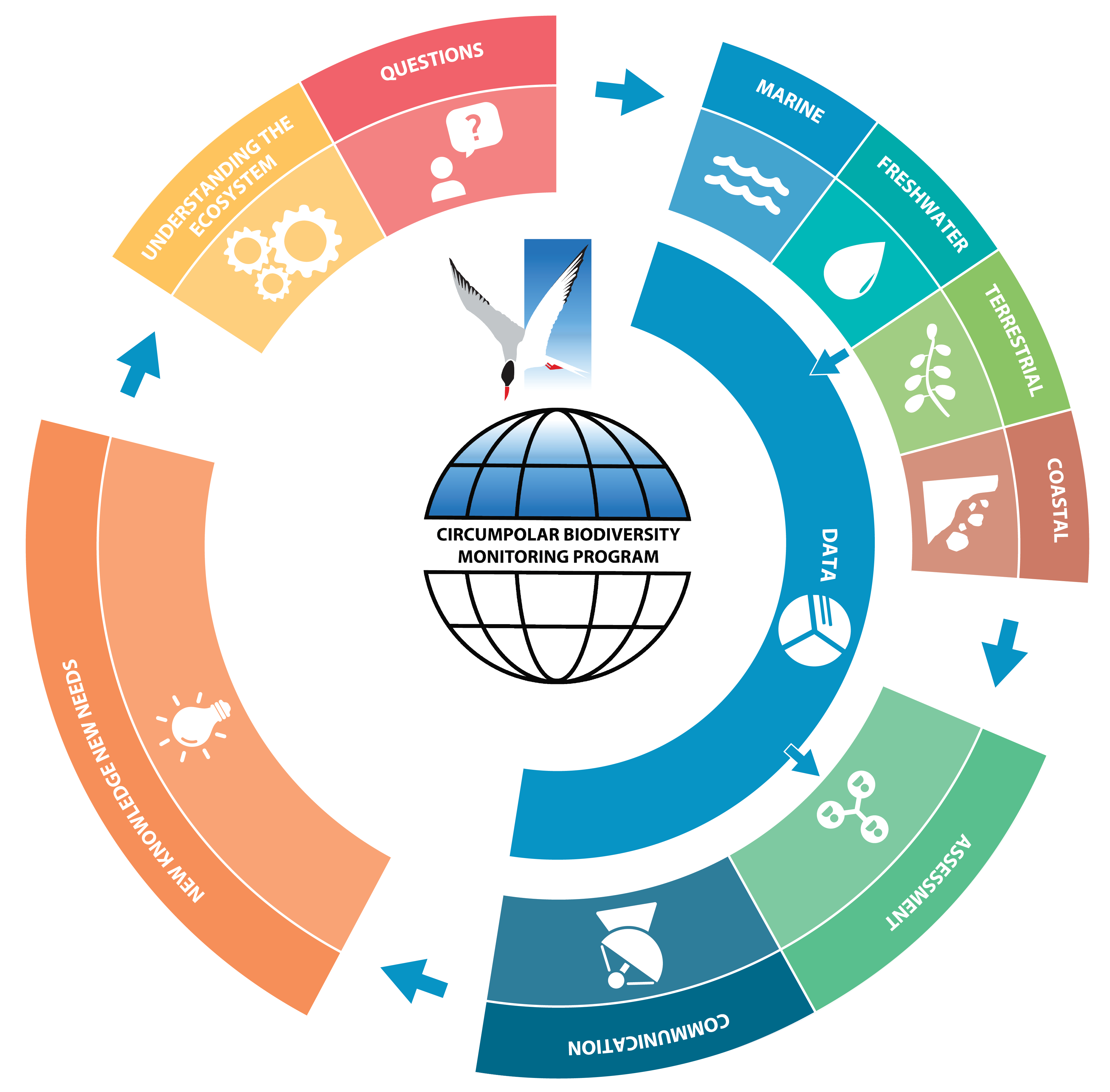
Figure 1-1. CBMP’s adaptive, integrated ecosystem–based approach to inventory, monitoring and data management. This figure illustrates how management questions, conceptual ecosystem models based on science, Indigenous Knowledge, and Local Knowledge, and existing monitoring networks guide the four CBMP monitoring plans––marine, freshwater, terrestrial and coastal. Monitoring outputs (data) feed into the assessment and decision-making processes and guide refinement of the monitoring programmes themselves. Modified from CAFF 2017 STATE OF THE ARCTIC TERRESTRIAL BIODIVERSITY REPORT - Chapter 1 - Page 4 - Figure 1-1
-
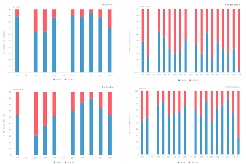
Time series of relative proportions of Arctic and Atlantic Calanus species in Kongsfjorden (top) and Rijpfjorden (bottom) (Source: MOSJ, Norwegian Polar Institute). STATE OF THE ARCTIC MARINE BIODIVERSITY REPORT - <a href="https://arcticbiodiversity.is/findings/plankton" target="_blank">Chapter 3</a> - Page 77 - Figure 3.2.8
-
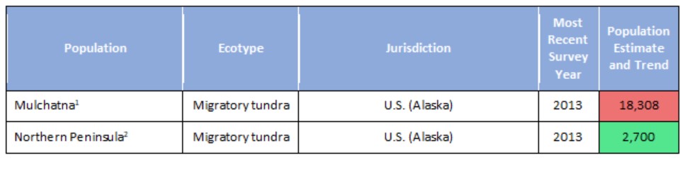
Population estimates and trends for Rangifer populations of the migratory tundra, Arctic island, mountain, and forest ecotypes where their circumpolar distribution intersects the CAFF boundary. Population trends (Increasing, Stable, Decreasing, or Unknown) are indicated by shading. Data sources for each population are indicated as footnotes. STATE OF THE ARCTIC TERRESTRIAL BIODIVERSITY REPORT - Chapter 3 - Page 70 - Table 3.4
-
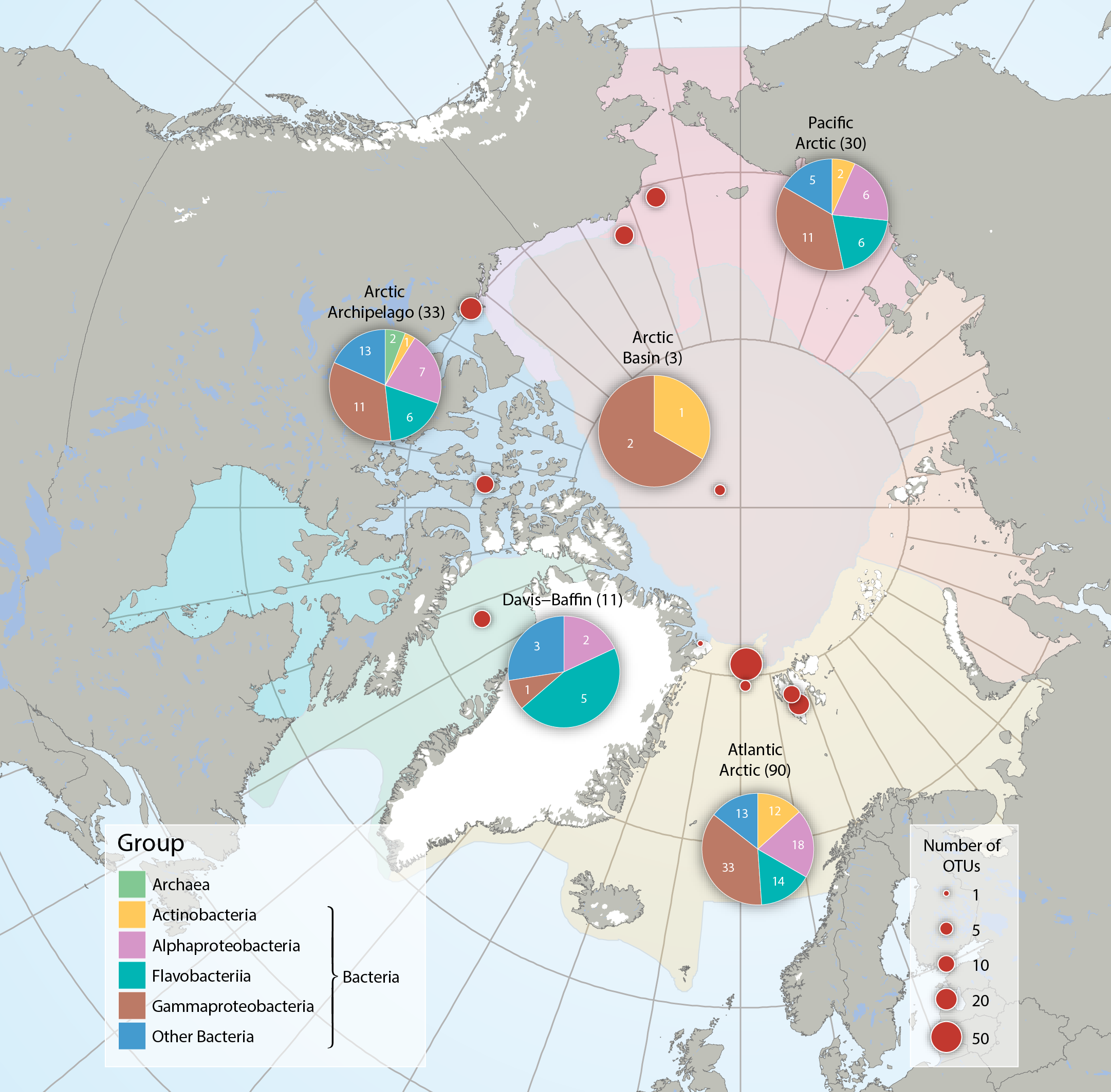
Bacteria and Archaea across five Arctic Marine Areas based on number of operational taxonomic units (OTUs), or molecular species. Composition of microbial groups, with respective numbers of OTUs (pie charts) and number of OTUs at sampling locations (red dots). Data aggregated by the CBMP Sea Ice Biota Expert Network. Data source: National Center for Biotechnology Information’s (NCBI 2017) Nucleotide and PubMed databases. STATE OF THE ARCTIC MARINE BIODIVERSITY REPORT - <a href="https://arcticbiodiversity.is/findings/sea-ice-biota" target="_blank">Chapter 3</a> - Page 38 - Figure 3.1.2 From the report draft: "Synthesis of available data was performed by using searches conducted in the National Center for Biotechnology Information’s “Nucleotide” (http://www.ncbi.nlm.nih.gov/guide/data-software/) and “PubMed” (http://www.ncbi.nlm.nih.gov/pubmed) databases. Aligned DNA sequences were downloaded and clustered into OTUs by maximum likelihood phylogenetic placement."
-
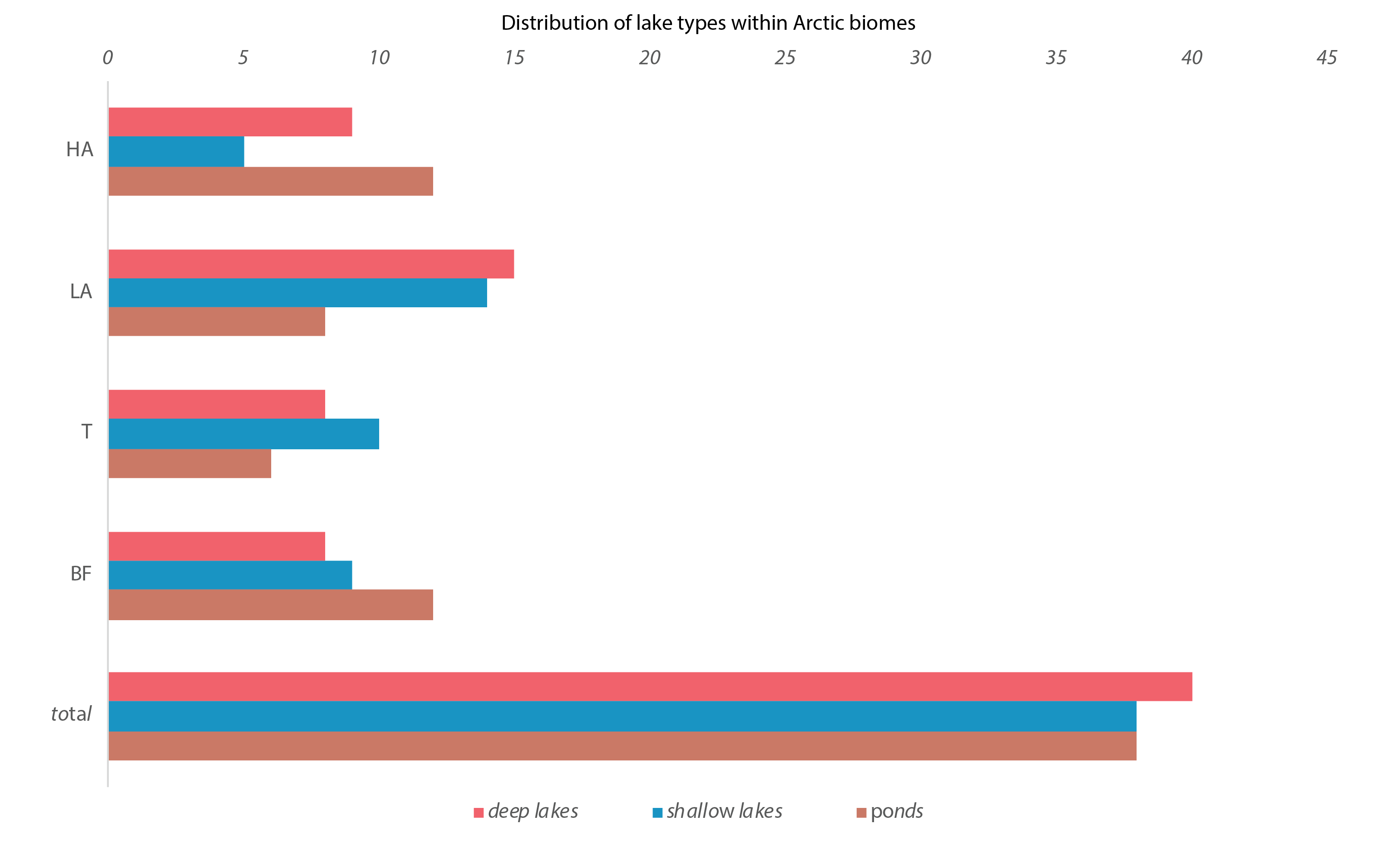
Figure 4-13 Number of deep lakes (red), shallow lakes (blue), and ponds (brown) in each geographical zone (BF, T, LA, HA). BF = Boreal Forest, T =Transition Zone, LA = Low Arctic, HA = High Arctic. State of the Arctic Freshwater Biodiversity Report - Chapter 4 - Page 40 - Figure 4-13
-
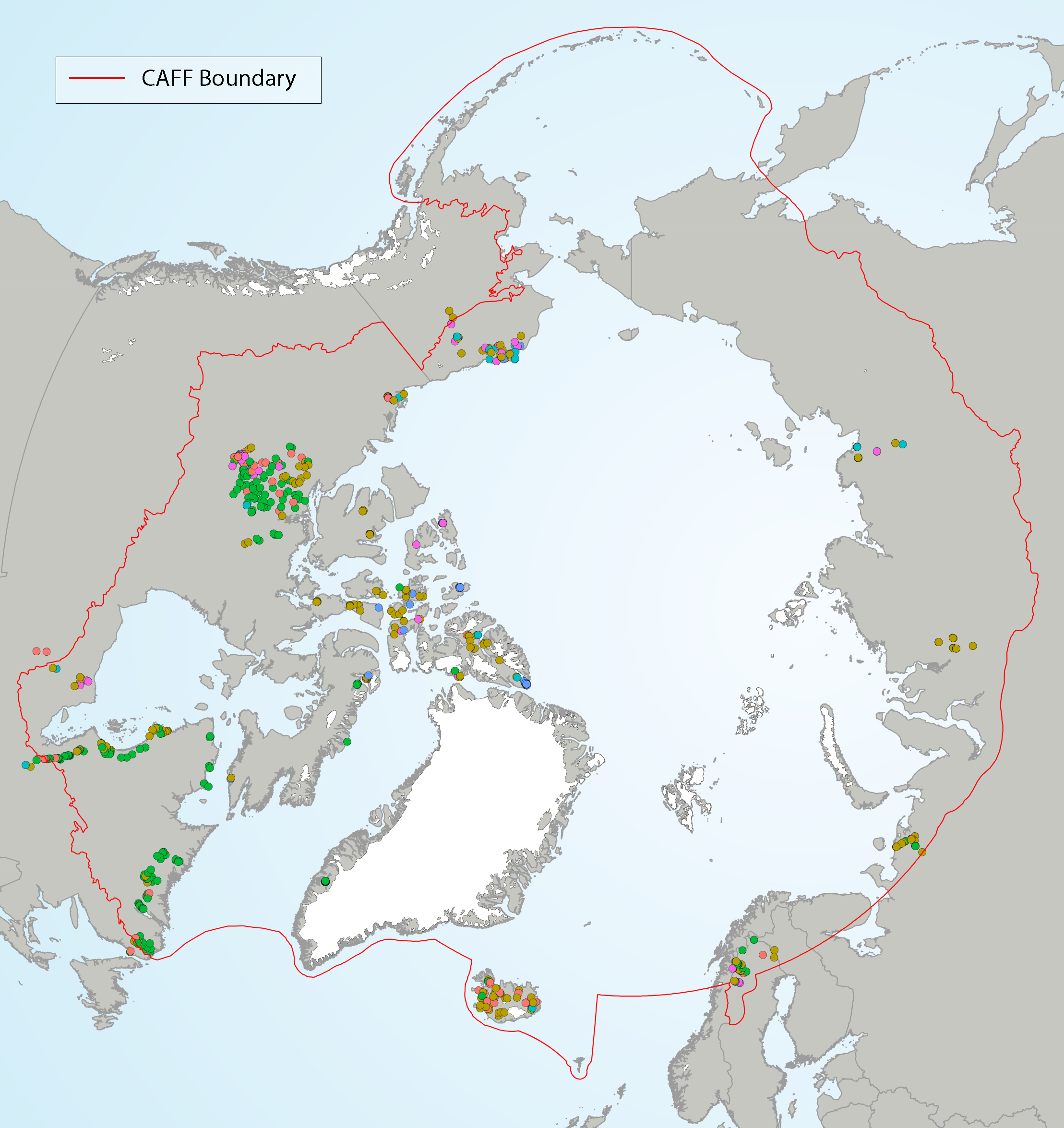
Figure 4 12 Diatom groups from Self Organizing Maps (SOMs) in lake top sediments, showing the geographical distribution of each group (with colors representing different SOM groups). State of the Arctic Freshwater Biodiversity Report - Chapter 4 - Page 39 - Figure 4-12
-
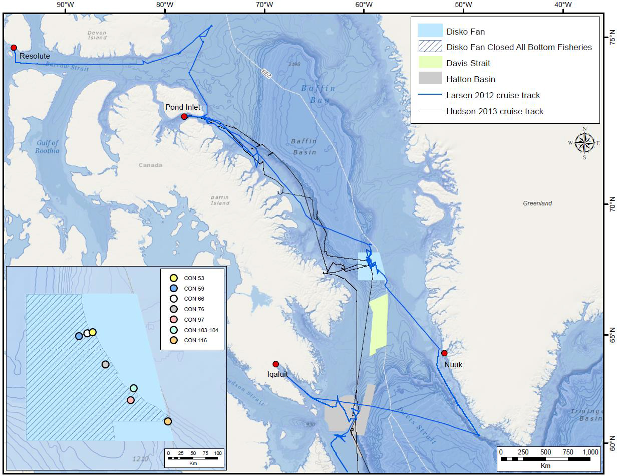
In 2012 and 2013, Fisheries and Oceans Canada conducted benthic imagery surveys in the Davis Strait and Baffin Basin in two areas then closed to bottom fishing, the Hatton Basin Voluntary Closure (now the Hatton Basin Conservation Area) and the Narwhal Closure (now partially in the Disko Fan Conservation Area). The photo transects were established as long-term biodiversity monitoring sites to monitor the impact of human activity, including climate change, on the region’s benthic marine biota in accordance with the protocols of the Circumpolar Biodiversity Monitoring Program established by the Council of Arctic Flora and Fauna. These images were analyzed in a techncial report that summarises the epibenthic megafauna found in seven image transects from the Disko Fan Conservation Area. A total of 480 taxa were found, 280 of which were identified as belonging to one of the following phyla: Annelida, Arthropoda, Brachiopoda, Bryozoa, Chordata, Cnidaria, Echinodermata, Mollusca, Nemertea, and Porifera. The remaining 200 taxa could not be assigned to a phylum and were categorised as Unidentified. Each taxon was identified to the lowest possible taxonomic level, typically class, order, or family. The summaries for each of the taxa include their identification numbers in the World Register of Marine Species and Integrated Taxonomic Information System’s databases, taxonomic hierarchies, images, and written descriptions. The report is intended to provide baseline documentation of the epibenthic megafauna in the Disko Fan Conservation Area, and serve as a taxonomic resource for future image analyses in the Arctic. Baker, E., Beazley, L., McMillan, A., Rowsell, J. and Kenchington, E. 2018. Epibenthic Megafauna of the Disko Fan Conservation Area in the Davis Strait (Eastern Arctic) Identified from In Situ Benthic Image Transects. Can. Tech. Rep. Fish. Aquat. Sci. 3272: vi + 388 p.
-
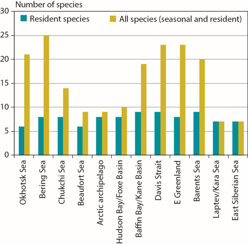
Number of marine mammal species in Arctic marine regions classified by resident species (n = 11 total) or all species (including seasonal visitors, n = 35 total). CAFF 2013. Arctic Biodiversity Assessment. Status and Trends in Arctic biodiversity. Conservation of Arctic Flora and Fauna, Akureyri - Mammal (Chapter 3) page 84