 CAFF - Arctic Biodiversity Data Service (ABDS)
Type of resources
Available actions
Topics
Keywords
Contact for the resource
Provided by
Years
Formats
Representation types
Update frequencies
status
Service types
Scale
-
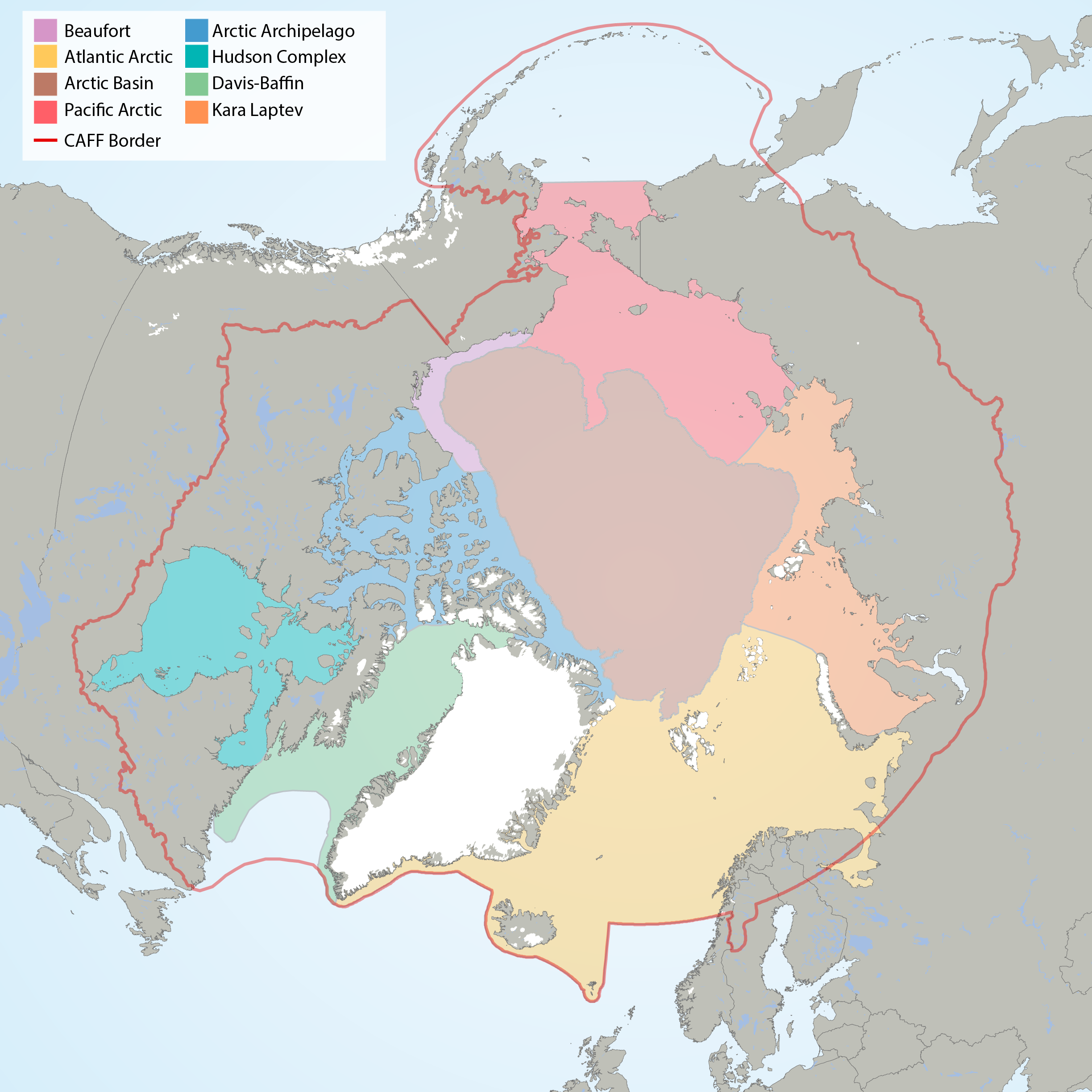
Arctic Marine Areas (AMAs) as defined in the CBMP Marine Plan. STATE OF THE ARCTIC MARINE BIODIVERSITY REPORT - <a href="https://arcticbiodiversity.is/marine" target="_blank">Chapter 1</a> - Page 15 - Figure 1.2
-
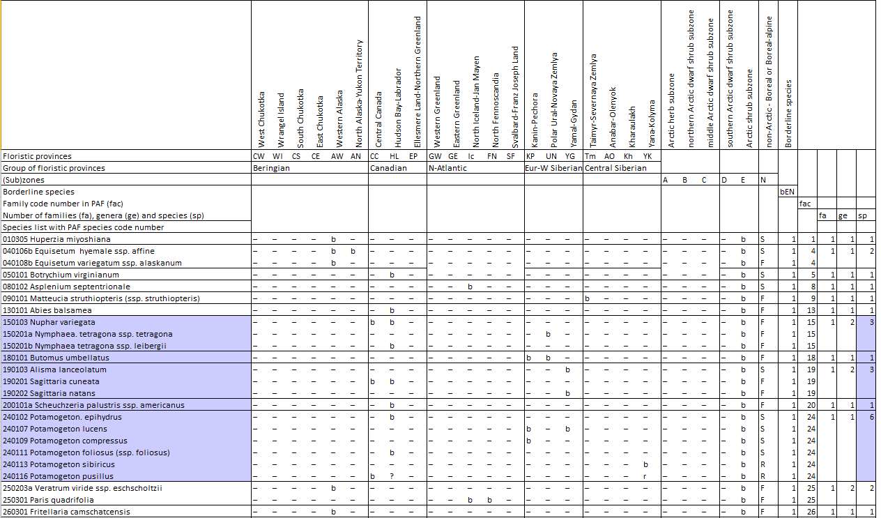
Appendix 9.3 Borderline vascular plant species (“b”) with indication of PAF code number, reaching the southernmost part of the Arctic subzone E. Arctic floristic provinces, subzones (A-E), neighbouring boreal or boreo-alpine zone (N) derived from Elven (2007).
-
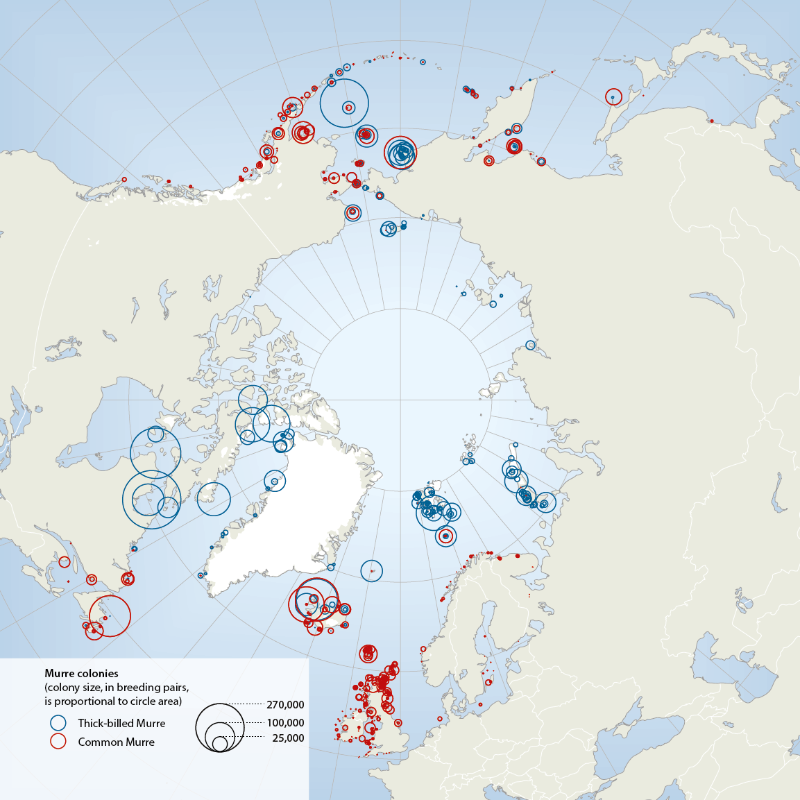
The two species of murres, thick-billed Uria lomvia and common U. aalge, both have circumpolar distributions, breeding in Arctic, sub-Arctic and temperate seas from alifornia and N Spain to N Greenland, high Arctic Canada, Svalbard, Franz Josef Land and Novaya Zemlya (Box 4.3 Fig. 1). Conservation of Arctic Flora and Fauna, CAFF 2013 - Akureyri . Arctic Biodiversity Assessment. Status and Trends in Arctic biodiversity. - Birds(Chapter 4) page 163
-
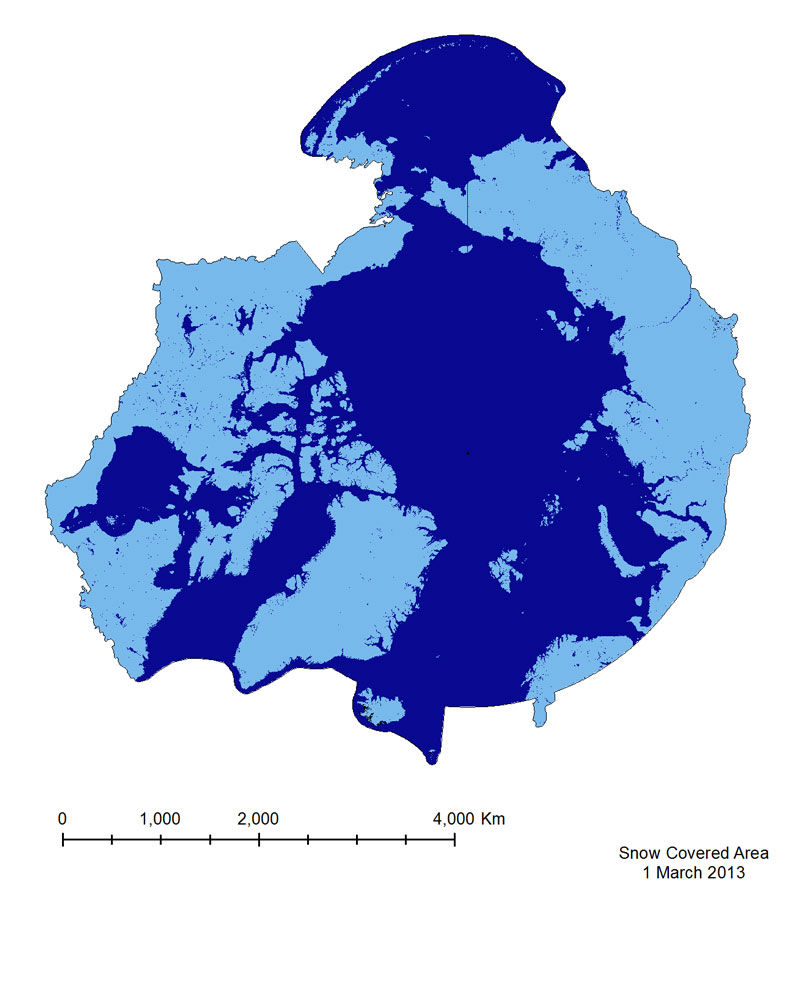
The Snow Covered Area product is based on a Normalized Difference Snow Index(NDSI), which is similar to NDVI, but exploits different bands in the equation (Equation 3),namely Green (Band 4) and Short Wavelength Near-infrared (SWNIR, Band 6). It isimportant to note that the Band 6 sensor on MODIS Aqua malfunctioned shortly after launch,so Snow Covered Area from the Aqua sensor is calculated using Bands 3 and 7. This mayintroduce errors in identifying snow in vegetated areas, as the use of Band 7 results in falsesnow detection. For this reason the MODIS Terra product has been provided for the CAFF-system.
-
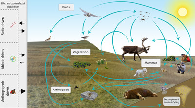
The Arctic terrestrial food web includes the exchange of energy and nutrients. Arrows to and from the driver boxes indicate the relative effect and counter effect of different types of drivers on the ecosystem. STATE OF THE ARCTIC TERRESTRIAL BIODIVERSITY REPORT - Chapter 2 - Page 26- Figure 2.4
-
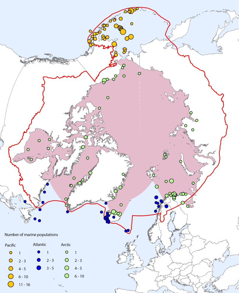
<img src="http://geo.abds.is/geonetwork/srv/eng//resources.get?uuid=59d822e4-56ce-453c-b98d-40207a2e9eec&fname=cbmp_small.png" alt="logo" height="67px" align="left" hspace="10px"> The Arctic marine data set contains a total of 111 species and 310 population time series from 170 locations. Species coverage is about 34% of Arctic marine vertebrate species (100% of mammals, 53% of birds, and 27% of fishes) (Bluhm et al. 2011). At the species level, even though the representation of Arctic fish species is lower than that of mammals and birds, the data are dominated by fishes, primarily from the Pacific Ocean (especially the Bering Sea and Aleutian Islands). However, there are more population time series in total for bird species, which is reflective of this group being both better studied historically and also monitored at many small study sites compared to fish and marine mammal species, which are regularly monitored at a much larger scale through stock management. Note that the time span selected for marine analyses is 1970 to 2005 (compared with 1970 to 2007 for the ASTI for all species). CAFF Assessment Series No. 7 April 2012 - <a href=http://caff.is/asti/asti-publications/28-arctic-species-trend-index-tracking-trends-in-arctic-marine-populations" target="_blank"> The Arctic Species Trend Index - Tracking trends in Arctic marine populations </a>
-
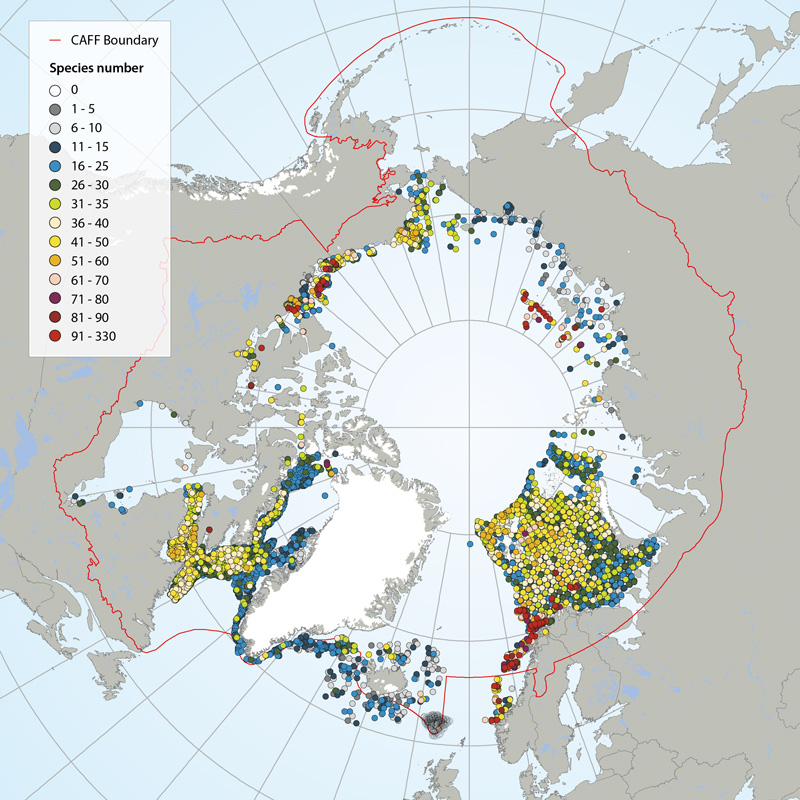
Number of megafauna species/taxa in the Arctic (7,322 stations in total), based on recent trawl investigations. Stations with highest species/taxon number are sorted to the top, meaning that dense concentrations of stations (e.g. Eastern Canada, Barents Sea), with low species numbers are hidden behind stations with higher species numbers. Also note that species numbers are somewhat biased by differing taxonomic resolution between studies. Data from: Icelandic Institute of Natural History, Iceland; Marine Research Institute, Iceland; University of Alaska, Fairbanks, U.S.; Greenland Institute of Natural Resources, Greenland; Zoological Institute of the Russian Academy of Sciences, St. Petersburg, Russia; Université du Québec à Rimouski, Canada; Fisheries and Oceans Canada; Institute of Marine Research, Norway; and Polar Research Institute of Marine Fisheries and Oceanography, Murmansk, Russia. STATE OF THE ARCTIC MARINE BIODIVERSITY REPORT - <a href="https://arcticbiodiversity.is/findings/benthos" target="_blank">Chapter 3</a> - Page 91 - Box figure 3.3.2 Several regions of the Pan Arctic have been sampled with trawl. Even though the trawl configurations and the taxonomic level are different from area to area, we choose to consider the taxonomic richness as relatively comparative.
-
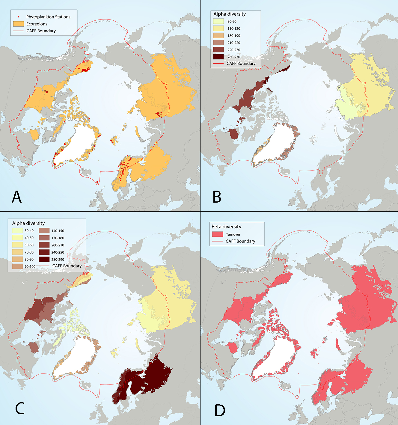
Figure 4 17 Results of circumpolar assessment of lake phytoplankton,(a) the location of phytoplankton stations, underlain by circumpolar ecoregions; (b) ecoregions with many phytoplankton stations, colored on the basis of alpha diversity rarefied to 35 stations; (c) all ecoregions with phytoplankton stations, colored on the basis of alpha diversity rarefied to 10 stations; (d) ecoregions with at least two stations in a hydrobasin, colored on the basis of the dominant component of beta diversity (species turnover, nestedness, approximately equal contribution, or no diversity) when averaged across hydrobasins in each ecoregion. State of the Arctic Freshwater Biodiversity Report - Chapter 4 - Page 56 - Figure 4-17
-
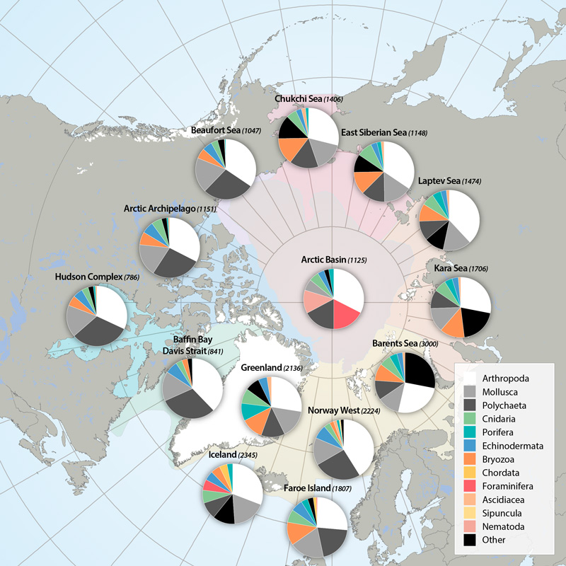
Arthropods (e.g., shrimps, crabs, sea spiders, amphipods, isopods) dominate taxon numbers in all Arctic regions, followed by polychaetes (e.g., bristle worms) and mollusks (e.g., gastropods, bivalves). Other taxon groups are diverse in some regions, such as bryozoans in the Kara Sea, cnidarians in the Atlantic Arctic, and foraminiferans in the Arctic deep-sea basins. This pattern is biased, however, by the meiofauna inclusion for the Arctic Basin (macro- and meiofauna size ranges overlap substantially in deep-sea fauna, so nematodes and foraminiferans are included) and the influence of a lack of specialists for some difficult taxonomic groups. STATE OF THE ARCTIC MARINE BIODIVERSITY REPORT - <a href="https://arcticbiodiversity.is/findings/benthos" target="_blank">Chapter 3</a> - Page 89 - Box figure 3.3.1 Each region of the Pan Arctic has been sampled with a set of different sampling gears, including grab, sledge and trawl, while other areas has only been sampled with grab. Here is the complete species/taxa number and the % distribution of species/taxa in main phyla, per region of the Pan Arctic.
-
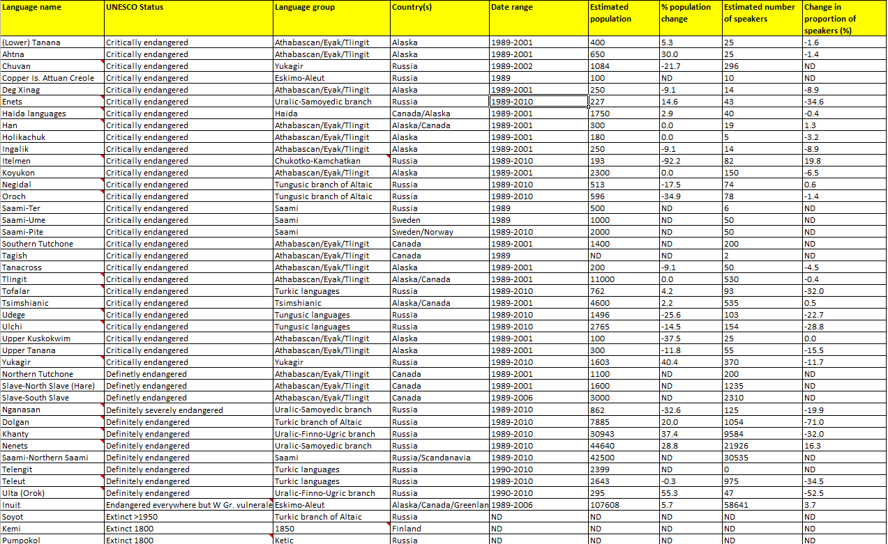
Appendix 20. Arctic indigenous languages status and trends. Data used to compile the information for the table was collected from both census records and academic sources, each of the CAFF countries and indigenous peoples organizations (Permanent Participants to the Arctic Council) where possible also provided statistical information.