 CAFF - Arctic Biodiversity Data Service (ABDS)
Land cover
Type of resources
Available actions
Topics
Keywords
Contact for the resource
Provided by
Years
Formats
Representation types
Update frequencies
status
-
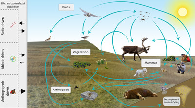
The Arctic terrestrial food web includes the exchange of energy and nutrients. Arrows to and from the driver boxes indicate the relative effect and counter effect of different types of drivers on the ecosystem. STATE OF THE ARCTIC TERRESTRIAL BIODIVERSITY REPORT - Chapter 2 - Page 26- Figure 2.4
-
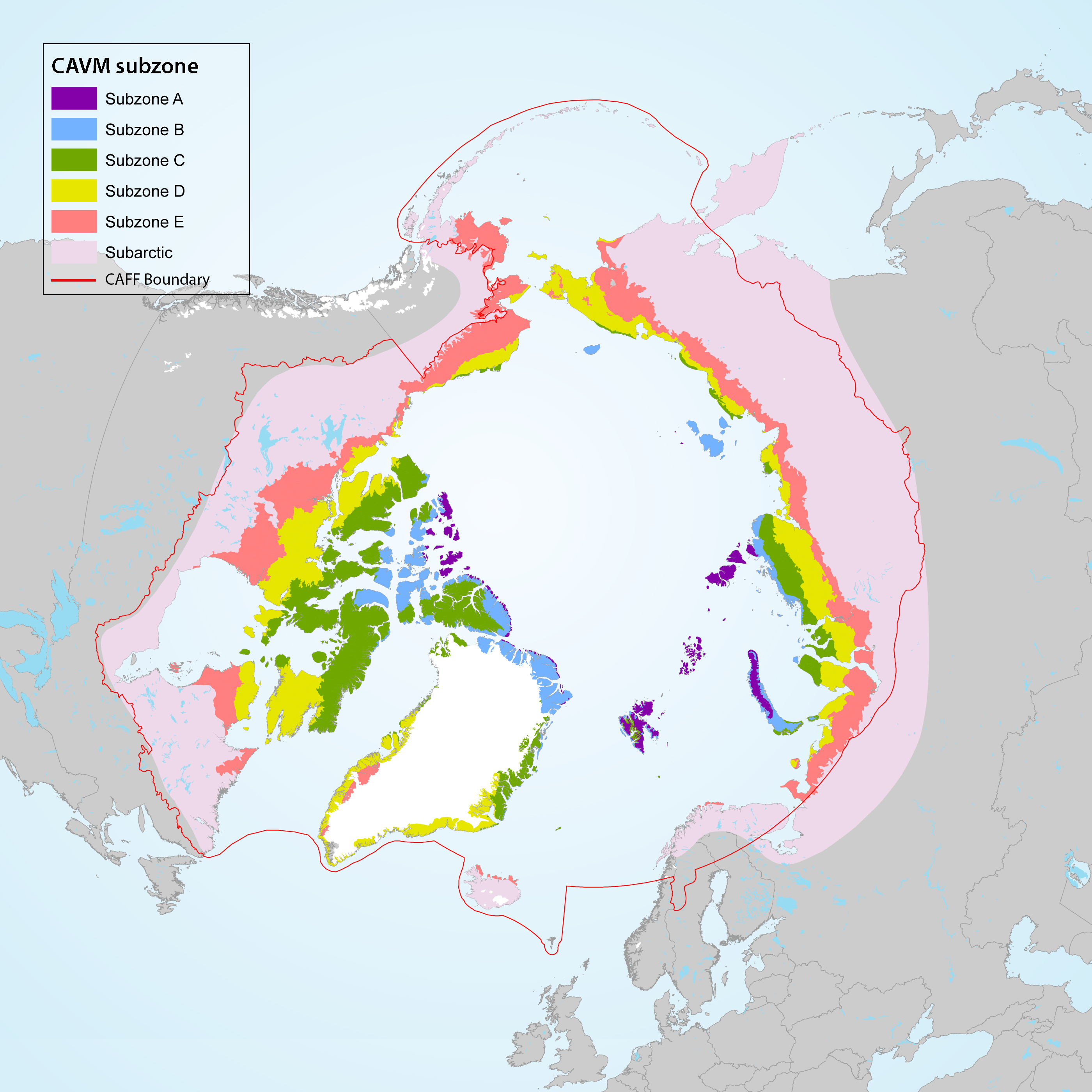
Geographic area covered by the Arctic Biodiversity Assessment and the CBMP–Terrestrial Plan. Subzones A to E are depicted as defined in the Circumpolar Arctic Vegetation Map (CAVM Team 2003). Subzones A, B and C are the high Arctic while subzones D and E are the low Arctic. Definition of high Arctic, low Arctic, and sub-Arctic follow Hohn & Jaakkola 2010. STATE OF THE ARCTIC TERRESTRIAL BIODIVERSITY REPORT - Chapter 1 - Page 14 - Figure 1.2
-
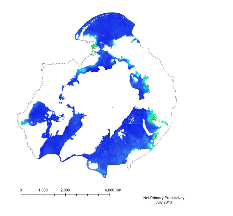
Marine primary productivity is not available from the NASA Ocean Color website. Currently the best product available for marine primary productivity is available through Oregon State University’s Ocean Productivity Project. A monthly global Net Primary Productivity product at 9 km spatial resolution has been selected for this analysis. The algorithm used to create the primary productivity is a Vertically Generalized Production Model (VGPM) created by Behrenfeld and Falkowski (1997). It is a “chlorophyll-based” model that estimates net primary production from chlorophyll using a temperature-dependent description of chlorophyll photosynthetic efficiency (O’Malley 2010). Inputs to the function are chlorophyll, available light, and photosynthetic efficiency.
-
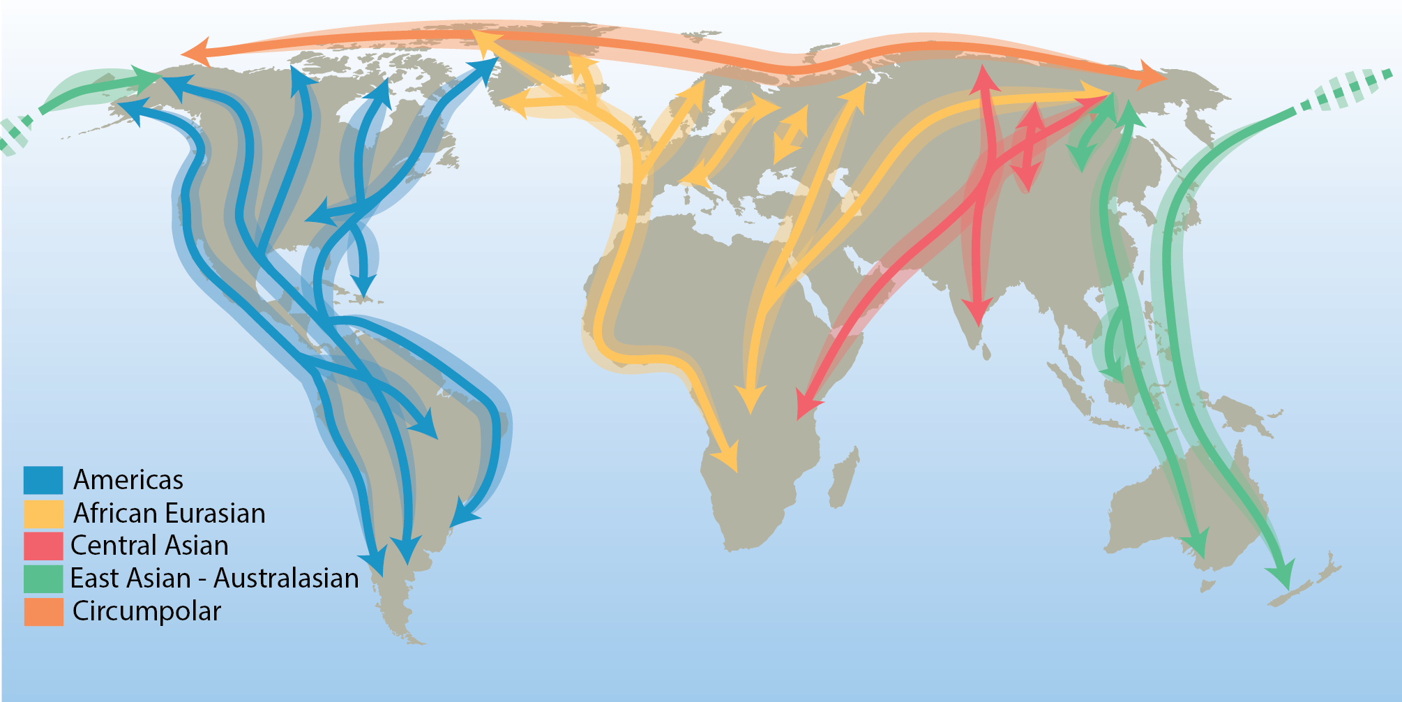
There are few true Arctic specialist birds that remain in the Arctic throughout their annual cycle. They include the willow and rock ptarmigan (Lagopus lagopus and L. muta), gyrfalcon (Falco rusticolus), snowy owl (Bubo scandiacus), Arctic redpoll (Carduelis hornemanni) and northern raven (Corvus corax)—a cosmopolitan species with resident populations in the Arctic. All other terrestrial Arctic-breeding bird species migrate to warmer regions during the northern winter, connecting the Arctic to all corners of the globe. Hence, their distributions are influenced by the routes they follow. These distinct migration routes are referred to as flyways and are defined by a combination of ecological and political boundaries and differ in spatial scale. The CBMP refers to the traditional four north–south flyways, in addition to a circumpolar flyway representing the few species that remain largely within the Arctic year-round (Figure 3-20). STATE OF THE ARCTIC TERRESTRIAL BIODIVERSITY REPORT - Chapter 3 - Page 48- Figure 3.20
-
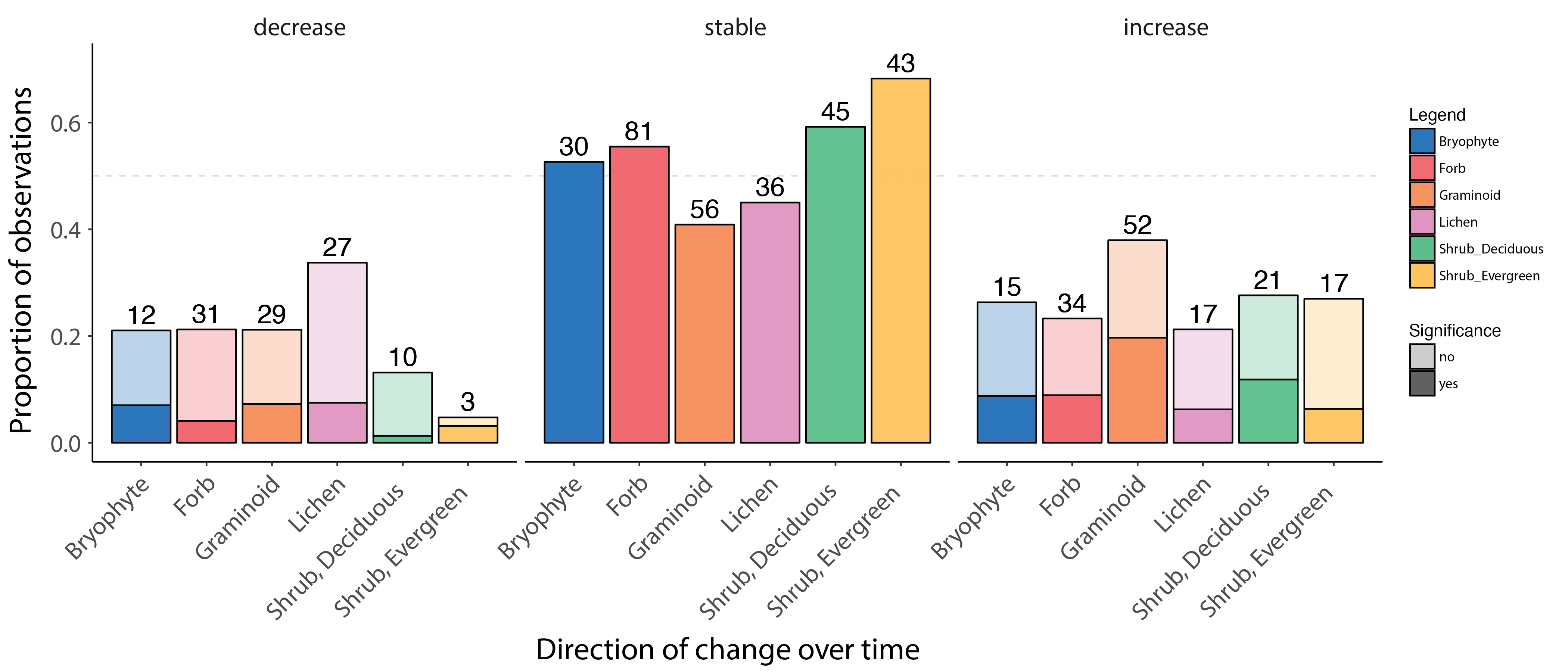
Change in forb, graminoid and shrub abundance by species or functional group over time based on local field studies across the Arctic, ranging from 5 to 43 years of duration. The bars show the proportion of observed decreasing, stable and increasing change in abundance, based on published studies. The darker portions of each bar represent a significant decrease, stable state, or increase, and lighter shading represents marginally significant change. The numbers above each bar indicate the number of observations in that group. Modified from Bjorkman et al. 2020. STATE OF THE ARCTIC TERRESTRIAL BIODIVERSITY REPORT - Chapter 3 - Page 31- Figure 3.2
-
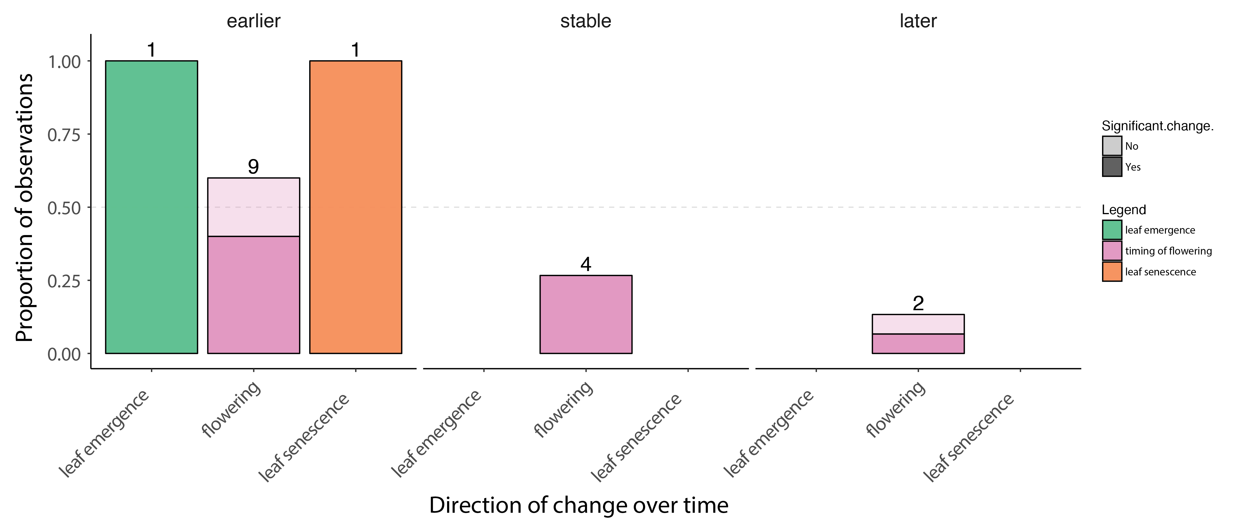
Change in plant phenology over time based on published studies, ranging from 9 to 21 years of duration. The bars show the proportion of observations where timing of phenological events advanced (earlier) was stable or were delayed (later) over time. The darker portions of each bar represent visible decrease, stable state, or increase results, and lighter portions represent marginally significant change. The numbers above each bar indicate the number of observations in that group. Figure from Bjorkman et al. 2020. STATE OF THE ARCTIC TERRESTRIAL BIODIVERSITY REPORT - Chapter 3 - Page 31- Figure 3.3
-
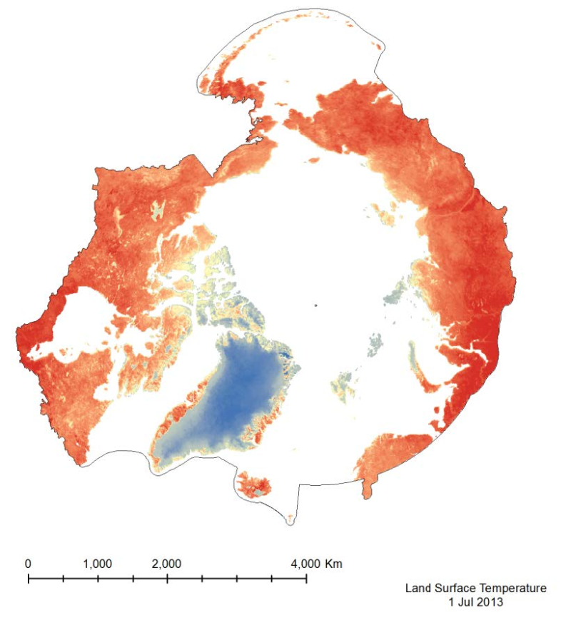
The MODIS Land Surface Temperature (LST) product provided is a monthlycomposite configured on a 0.05° Climate Model Grid (CMG). It includes both daytime andnighttime surface temperatures, taken at 11 um and 4 um (night). This product has beenscaled. To convert the raster values to a Kelvin temperature scale, multiply by a factor of 0.02.
-
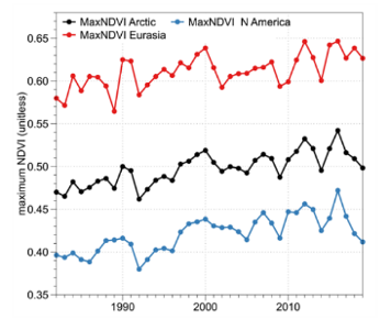
Circumpolar trends in primary productivity as indicated by the maximum Normalised Difference Vegetation Index, 1982–2017. (a) Brown shading indicates negative MaxNDVI trends, green shading indicates positive MaxNDVI trends. (b) Chart of trends for the circumpolar Arctic, Eurasia, and North America. Modified from Frost et al. 2020. STATE OF THE ARCTIC TERRESTRIAL BIODIVERSITY REPORT - Chapter 3 - Page 30 - Figure 3.1
-
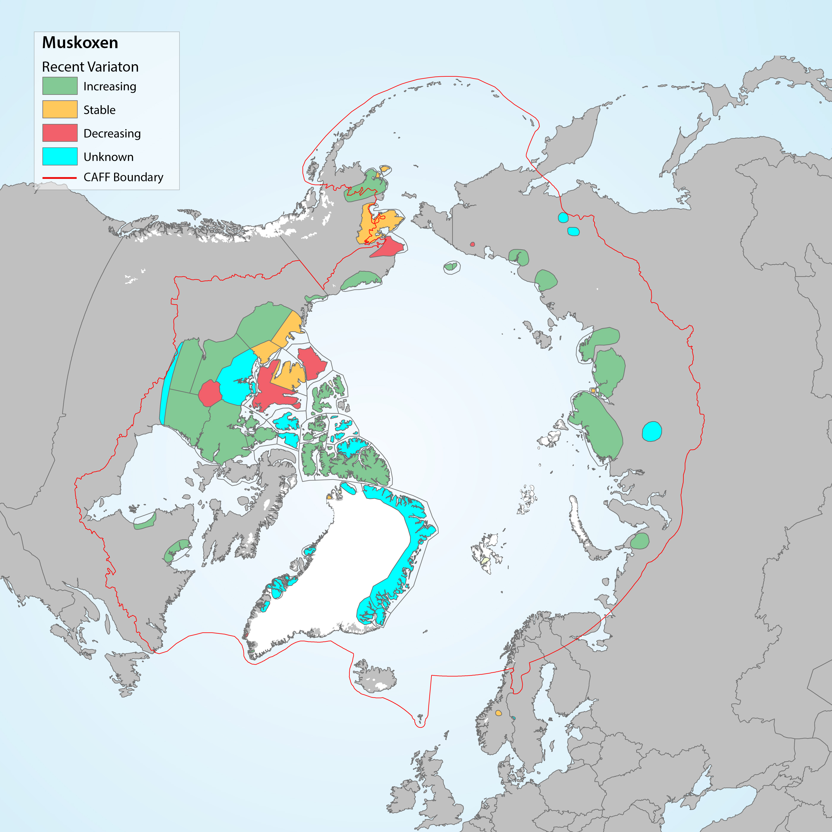
Trends and distribution of muskoxen populations based on Table 3-5. Modified from Cuyler et al. 2020. STATE OF THE ARCTIC TERRESTRIAL BIODIVERSITY REPORT - Chapter 3 - Page 79 - Figure 3.30
-
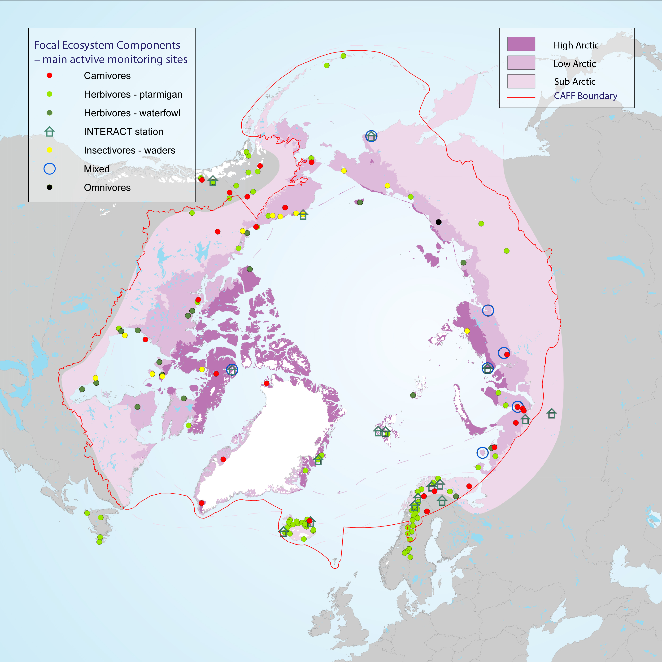
Many population counts of gregarious migrant species, such as waders and geese, take place along the flyways and at wintering grounds outside the Arctic which stresses the importance of continued development of movement ecology studies. Monitoring of FEC attributes related to breeding success and links to environmental drivers within the Arctic takes place in a wide network of research sites across the Arctic, although with low coverage of the high Arctic zone (Figure 3-25) STATE OF THE ARCTIC TERRESTRIAL BIODIVERSITY REPORT - Chapter 3 - Page 58 - Figure 3.25