 CAFF - Arctic Biodiversity Data Service (ABDS)
unknown
Type of resources
Available actions
Topics
Keywords
Contact for the resource
Provided by
Years
Formats
Representation types
Update frequencies
status
Scale
-
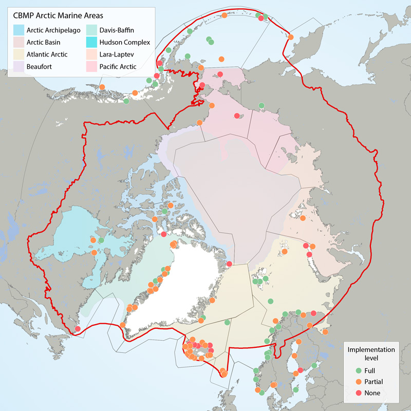
Boundaries of the 22 ecoregions (grey lines) as defined in the CSMP (Irons et al. 2015) and the Arctic Marine Areas (colored polygons with names in legend). Filled circles show locations of seabird colony sites recommended for monitoring (‘key sites’). The current level of monitoring plan implementation are green = fully implemented, amber = partially implemented, red = not implemented. The CSMP provides implementation maps for each forage guild. STATE OF THE ARCTIC MARINE BIODIVERSITY REPORT - <a href="https://arcticbiodiversity.is/findings/seabirds" target="_blank">Chapter 3</a> - Page 132 - Figure 3.5.1 This graphic displays the status of seabird monitoring at key sites in CBMP areas across the Arctic.
-
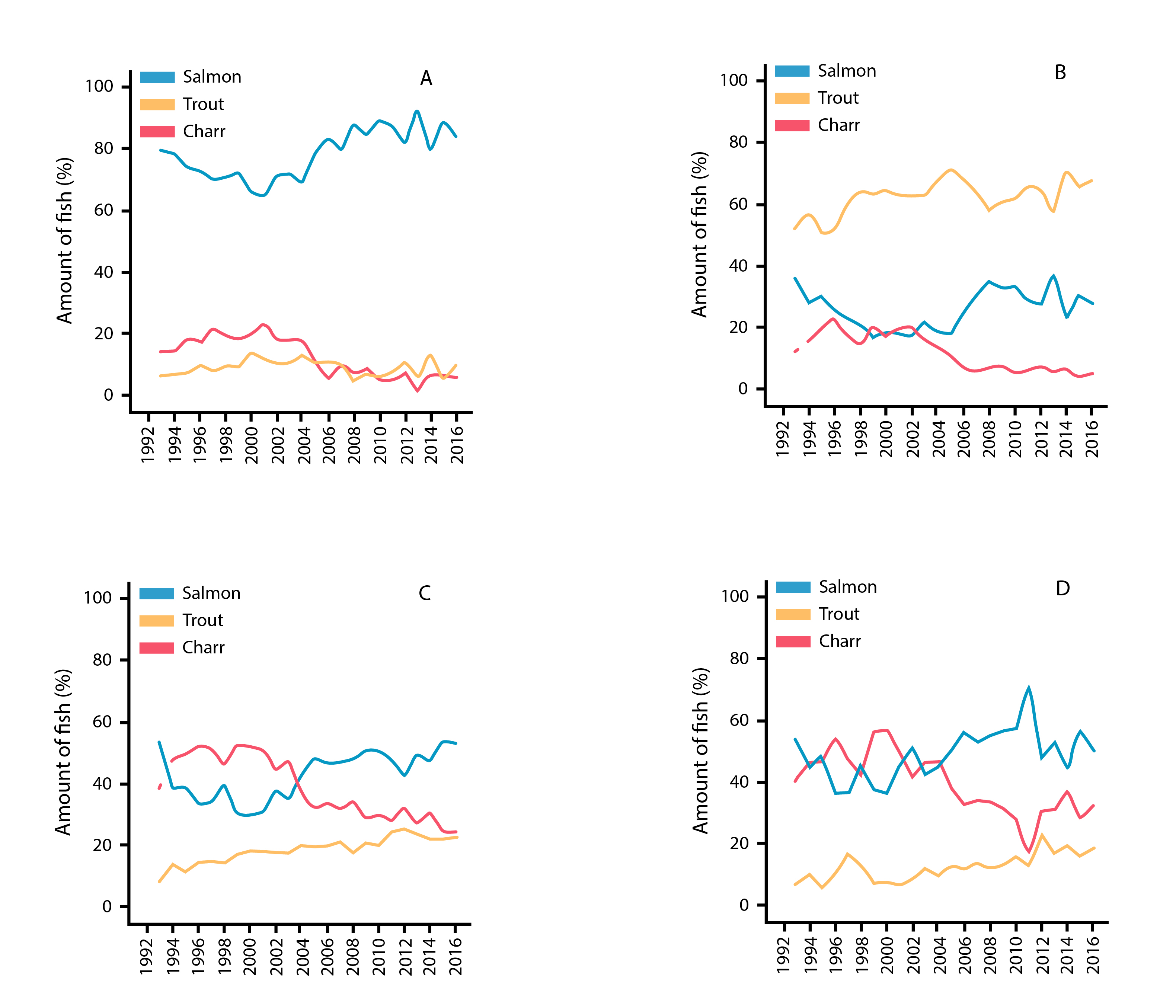
Temporal patterns in % abundance of Atlantic salmon, brown trout, and anadromous Arctic charr from catch statistics in Iceland rivers monitored from 1992 to 2016, showing results from (a) west, (b) south, (c) north, and (d) east Iceland. State of the Arctic Freshwater Biodiversity Report - Chapter 4 - Page 81 - Figure 4-41
-
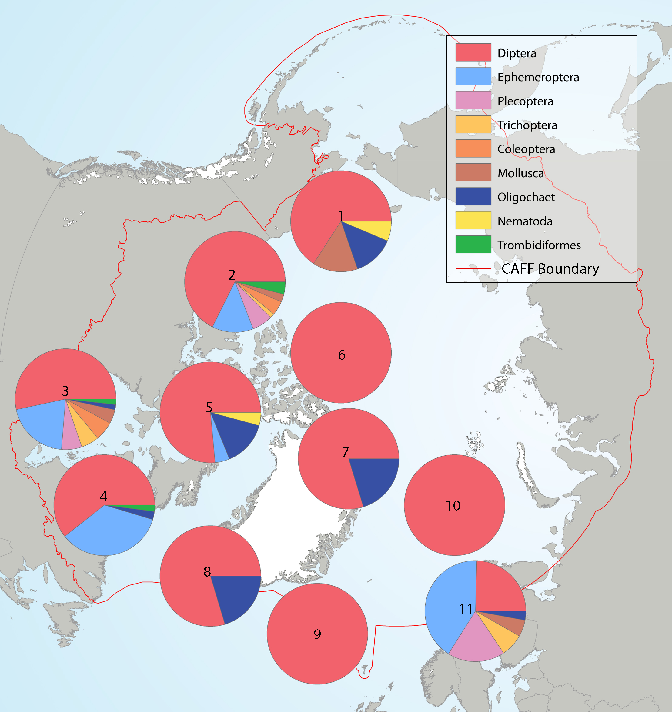
Summary of the taxa accounting for 85% of the river benthic macroinvertebrates collected in each of several highly-sampled geographic areas, with taxa grouped by order level or higher in pie charts placed spatially to indicate sampling area. Pie charts correspond to (1) Alaska, (2) western Canada, (3) southern Canada, south of Hudson Bay, (4) northern Labrador, (5) Baffin Island, (6) Ellesmere Island, (7) Greenland high Arctic, (8) Greenland low Arctic, (9) Iceland, (10) Svalbard, and (11) Fennoscandia. State of the Arctic Freshwater Biodiversity Report - Chapter 4 - Page 70 - Figure 4-34
-
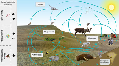
The Arctic terrestrial food web includes the exchange of energy and nutrients. Arrows to and from the driver boxes indicate the relative effect and counter effect of different types of drivers on the ecosystem. STATE OF THE ARCTIC TERRESTRIAL BIODIVERSITY REPORT - Chapter 2 - Page 26- Figure 2.4
-
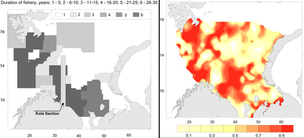
Commercial fishery impact on zoobenthos of the Barents Sea. Figure A) Intensity and duration of fishery efforts in standard commercial fishery areas in the Barents Sea. The darker the area the longer the fishery has been in operation. Figure B) Level of decline in macrobenthic biomass between 1926-1932 and 1968-1970 calculated as 1-b1968/b1930. The largest biomass decreases correspond to the darker colour, whereas lighter colour refers to no change (Denisenko 2013). STATE OF THE ARCTIC MARINE BIODIVERSITY REPORT - <a href="https://arcticbiodiversity.is/findings/benthos" target="_blank">Chapter 3</a> - Page 97 - Figure 3.3.4
-
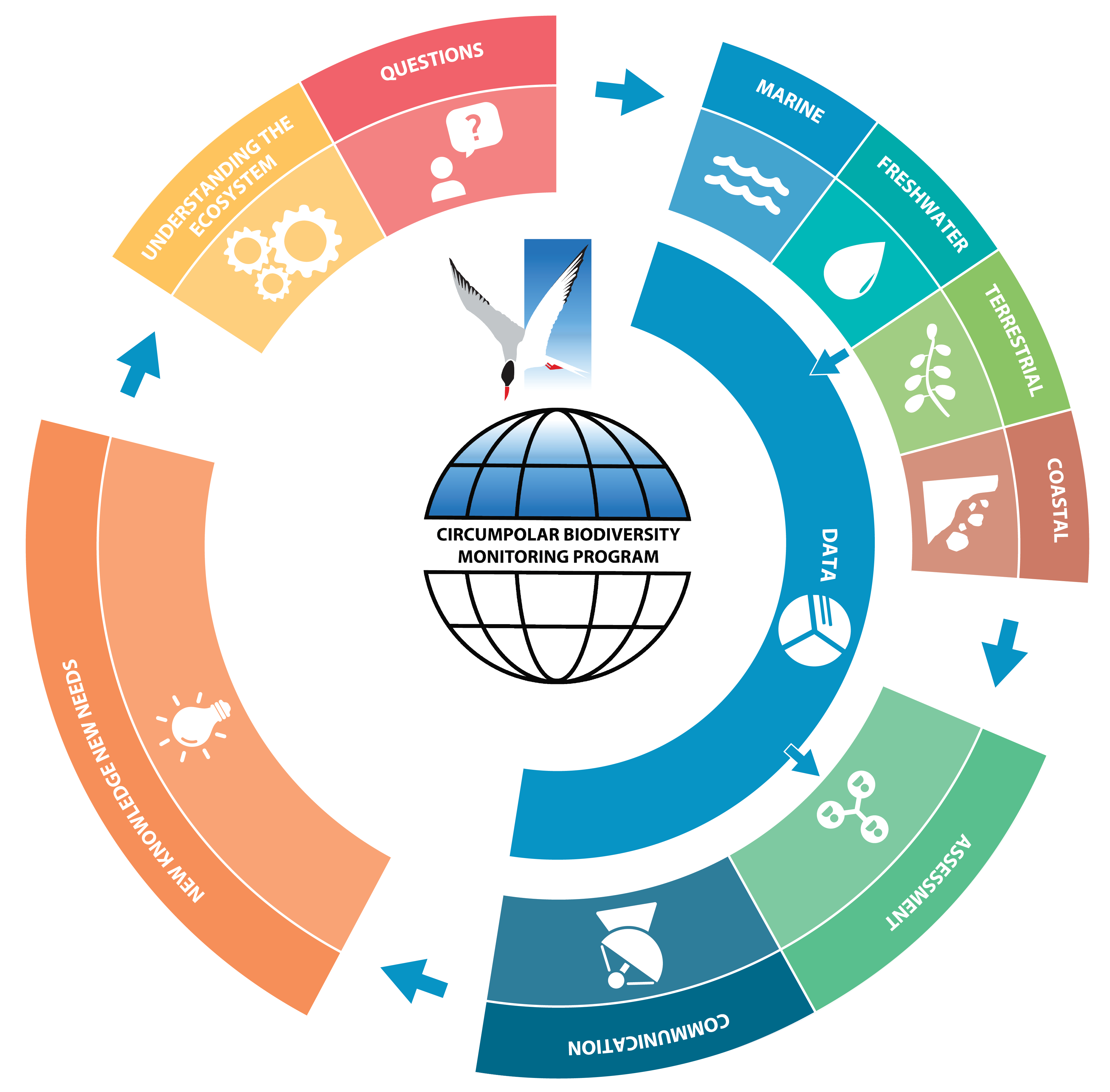
Figure 1-1. CBMP’s adaptive, integrated ecosystem–based approach to inventory, monitoring and data management. This figure illustrates how management questions, conceptual ecosystem models based on science, Indigenous Knowledge, and Local Knowledge, and existing monitoring networks guide the four CBMP monitoring plans––marine, freshwater, terrestrial and coastal. Monitoring outputs (data) feed into the assessment and decision-making processes and guide refinement of the monitoring programmes themselves. Modified from CAFF 2017 STATE OF THE ARCTIC TERRESTRIAL BIODIVERSITY REPORT - Chapter 1 - Page 4 - Figure 1-1
-
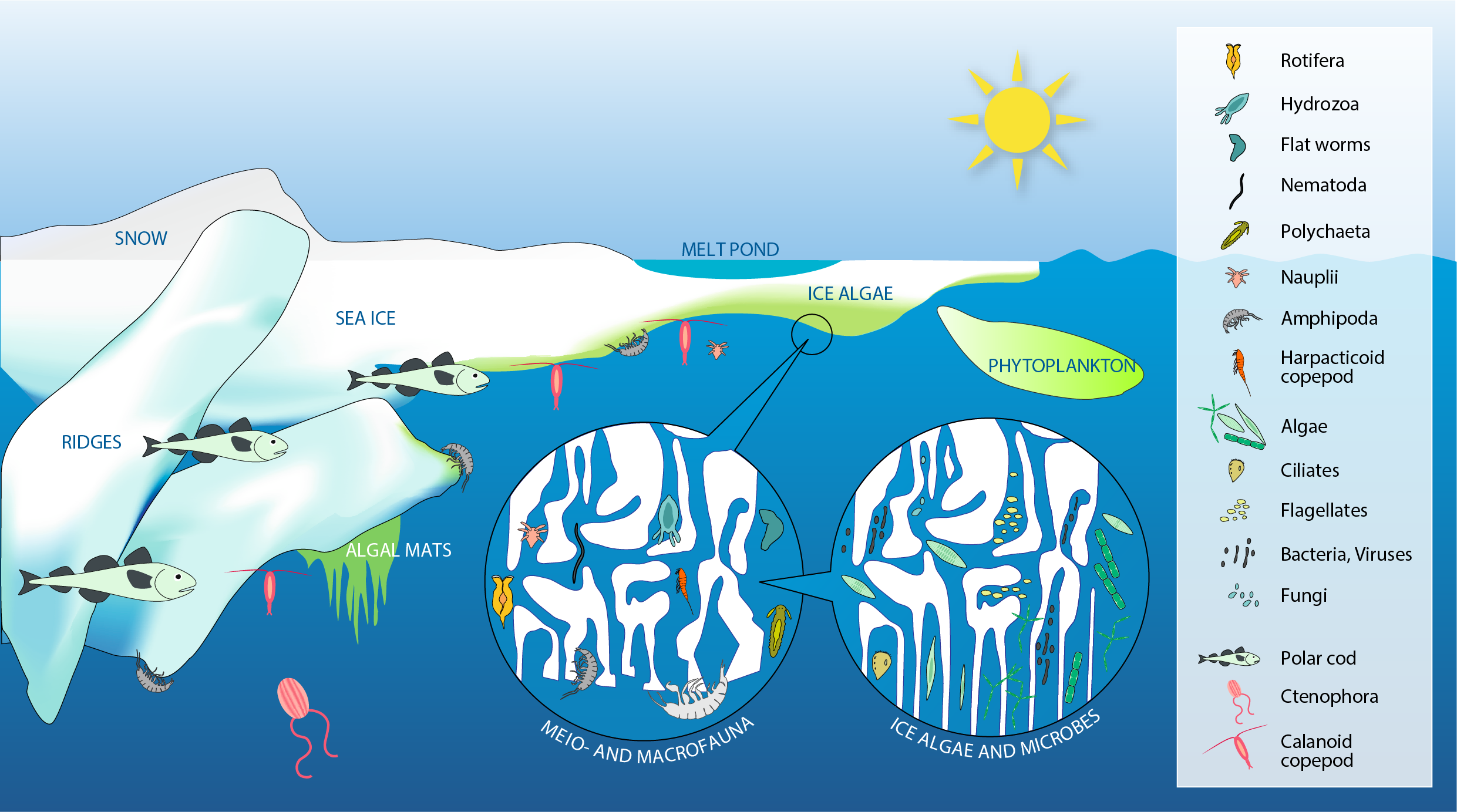
Sea ice provides a wide range of microhabitats for diverse biota including microbes, single-celled eukaryotes (labelled algae), multicellular meiofauna, larger under-ice fauna (represented by amphipods), as well as polar cod (Boreogadus saida). Modified from Bluhm et al. (2017). STATE OF THE ARCTIC MARINE BIODIVERSITY REPORT - <a href="https://arcticbiodiversity.is/findings/sea-ice-biota" target="_blank">Chapter 3</a> - Page 35 - Figure 3.1.1
-
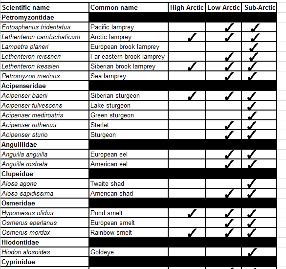
Appendix 6.1.1. Freshwater and diadromous fish species by area of occurrence within the High Arctic, Low Arctic and sub-Arctic. Appendix 6.1.2. Freshwater and diadromous fishes of the Palearctic and Nearctic regions. Appendix 6.1.3. Occurrence of freshwater and diadromous fishes in the Arctic and sub-Arctic regions of the seven geographical regions referred to in the main text. Appendix 6.1.4. Freshwater and diadromous fish species status summary for species assessed at some level of risk by country or region
-
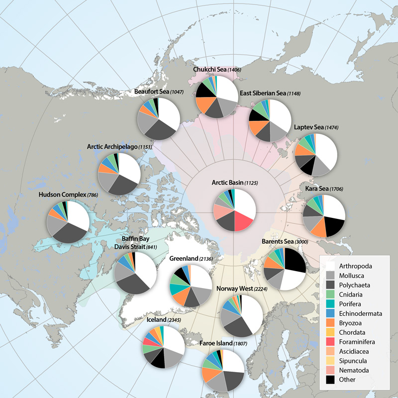
Arthropods (e.g., shrimps, crabs, sea spiders, amphipods, isopods) dominate taxon numbers in all Arctic regions, followed by polychaetes (e.g., bristle worms) and mollusks (e.g., gastropods, bivalves). Other taxon groups are diverse in some regions, such as bryozoans in the Kara Sea, cnidarians in the Atlantic Arctic, and foraminiferans in the Arctic deep-sea basins. This pattern is biased, however, by the meiofauna inclusion for the Arctic Basin (macro- and meiofauna size ranges overlap substantially in deep-sea fauna, so nematodes and foraminiferans are included) and the influence of a lack of specialists for some difficult taxonomic groups. STATE OF THE ARCTIC MARINE BIODIVERSITY REPORT - <a href="https://arcticbiodiversity.is/findings/benthos" target="_blank">Chapter 3</a> - Page 89 - Box figure 3.3.1 Each region of the Pan Arctic has been sampled with a set of different sampling gears, including grab, sledge and trawl, while other areas has only been sampled with grab. Here is the complete species/taxa number and the % distribution of species/taxa in main phyla, per region of the Pan Arctic.
-
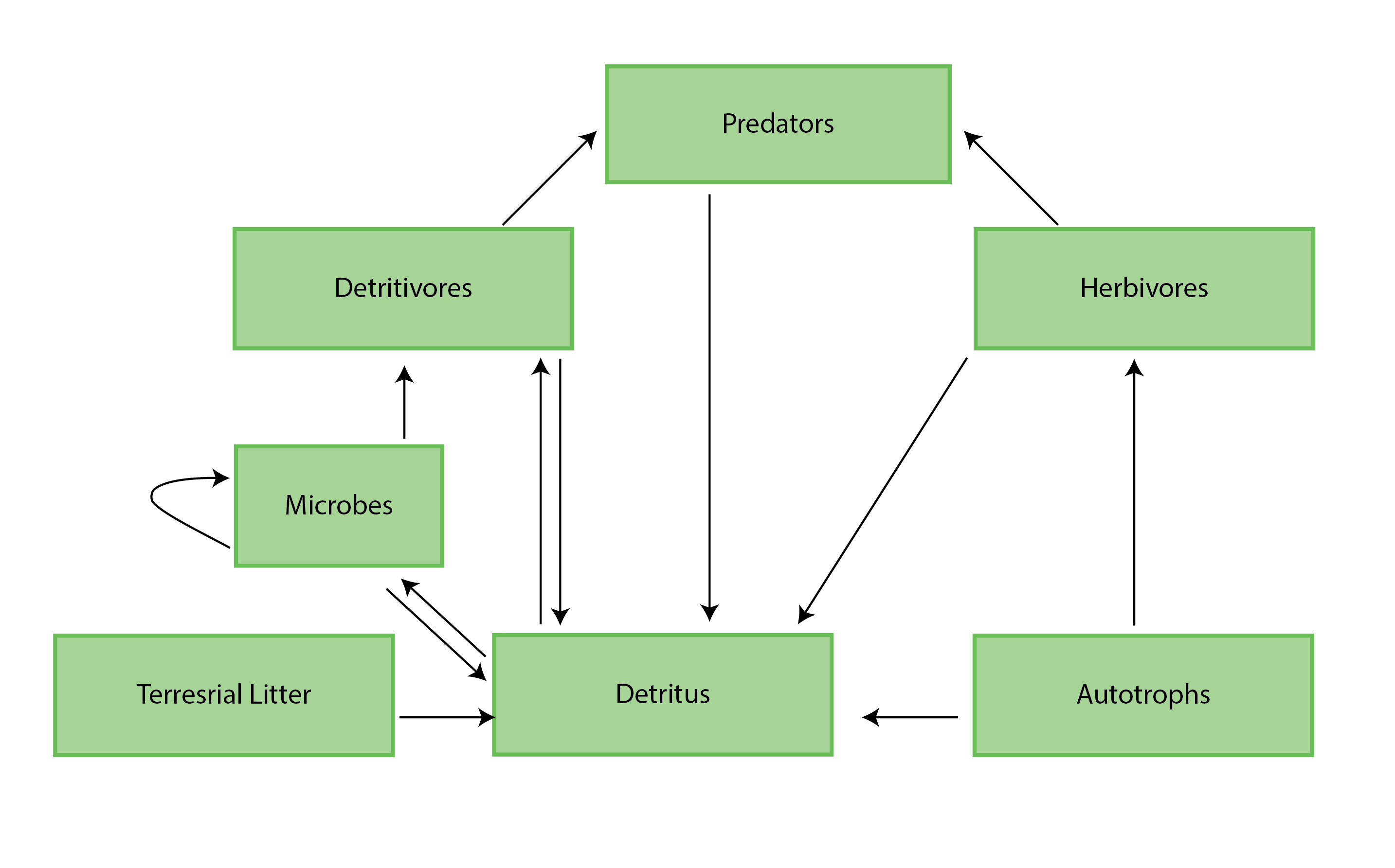
Figure 4-1 A generic food web diagram for a lake or river, indicating the basic trophic levels (boxes) and energy flow (arrows) between those levels. Reproduced from Culp et al. (2012a). State of the Arctic Freshwater Biodiversity Report - Chapter 4 - Page 25 - Figure 4-1