 CAFF - Arctic Biodiversity Data Service (ABDS)
unknown
Type of resources
Available actions
Topics
Keywords
Contact for the resource
Provided by
Years
Formats
Representation types
Update frequencies
status
Scale
-
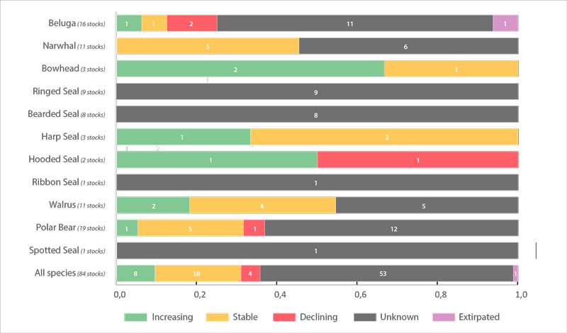
Trends in abundance of Arctic marine mammal Focal Ecosystem Components based on the most recent assessment for each recognized subpopulation of a species (red, declining trend; yellow, stable trend; green, increasing trend; grey, unknown trend). Number of subpopulations is given after species name. Each column is divided into equal segments, the sizes of which are not proportional to the size of the subpopulation. Ringed seal and bearded seal segments represent subspecies. Walrus segments represent subpopulations within subspecies. See Table 3.6.1 for details on abundance. STATE OF THE ARCTIC MARINE BIODIVERSITY REPORT - <a href="https://arcticbiodiversity.is/findings/marine-mammals" target="_blank">Chapter 3</a> - Page 156 - Figure 3.6.2
-
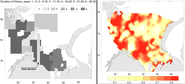
Commercial fishery impact on zoobenthos of the Barents Sea. Figure A) Intensity and duration of fishery efforts in standard commercial fishery areas in the Barents Sea. The darker the area the longer the fishery has been in operation. Figure B) Level of decline in macrobenthic biomass between 1926-1932 and 1968-1970 calculated as 1-b1968/b1930. The largest biomass decreases correspond to the darker colour, whereas lighter colour refers to no change (Denisenko 2013). STATE OF THE ARCTIC MARINE BIODIVERSITY REPORT - <a href="https://arcticbiodiversity.is/findings/benthos" target="_blank">Chapter 3</a> - Page 97 - Figure 3.3.4
-
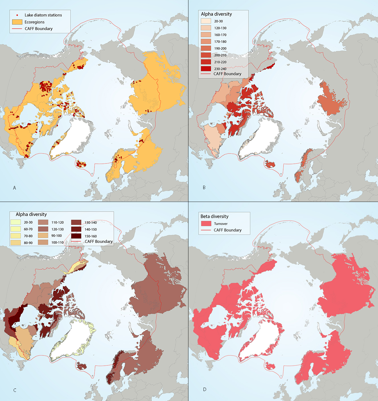
Figure 4-7 Circumpolar assessment of lake diatoms, indicating (a) the location of lake diatom stations, underlain by circumpolar ecoregions; (b) ecoregions with many lake diatom stations, colored on the basis of alpha diversity rarefied to 40 stations; (c) all ecoregions with lake diatom stations, colored on the basis of alpha diversity rarefied to 10 stations; (d) ecoregions with at least two stations in a hydrobasin, colored on the basis of the dominant component of beta diversity (i.e. species turnover, nestedness, approximately equal contribution, or no diversity) when averaged across hydrobasins in each ecoregio. State of the Arctic Freshwater Biodiversity Report - Chapter 4 - Page 35 - Figure 4-7
-
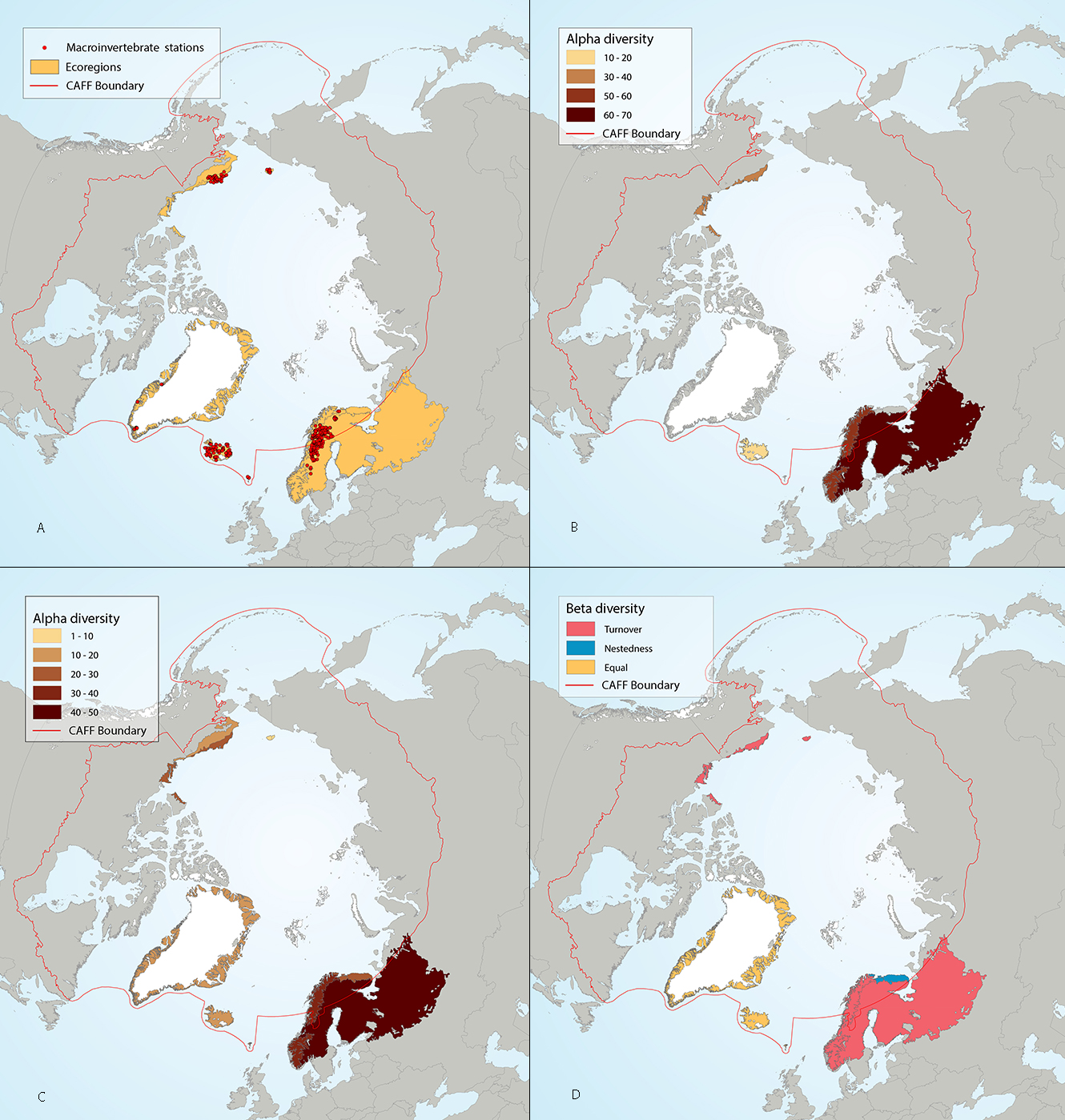
Results of circumpolar assessment of lake littoral benthic macroinvertebrates, indicating (a) the location of littoral benthic macroinvertebrate stations, underlain by circumpolar ecoregions; (b) ecoregions with many littoral benthic macroinvertebrate stations, colored on the basis of alpha diversity rarefied to 80 stations; (c) all ecoregions with littoral benthic macroinvertebrate stations, colored on the basis of alpha diversity rarefied to 10 stations; (d) ecoregions with at least two stations in a hydrobasin, colored on the basis of the dominant component of beta diversity (species turnover, nestedness, approximately equal contribution, or no diversity) when averaged across hydrobasins in each ecoregion. State of the Arctic Freshwater Biodiversity Report - Chapter 4 - Page 65 - Figure 4-29
-
The baseline survey and ongoing monitoring required to adequately describe Arctic arthropod biodiversity and to identify trends is largely lacking. Although some existing publications reporting long-term and extensive sampling exist, they are limited in species level information, taxonomic coverage and/or geographic location/extent (Figure 3-19) STATE OF THE ARCTIC TERRESTRIAL BIODIVERSITY REPORT - Chapter 3 - Page 44 - Figure 3.19
-
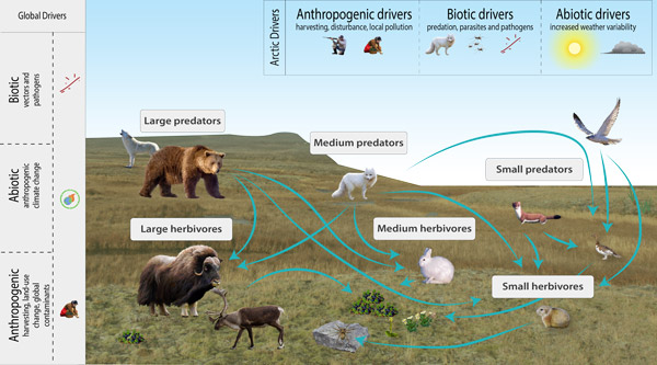
Conceptual model of Arctic terrestrial mammals, showing FECs, interactions with other biotic groups and examples of drivers and attributes relevant at various spatial scales. STATE OF THE ARCTIC TERRESTRIAL BIODIVERSITY REPORT - Chapter 3 - Page 67 - Figure 3.28
-
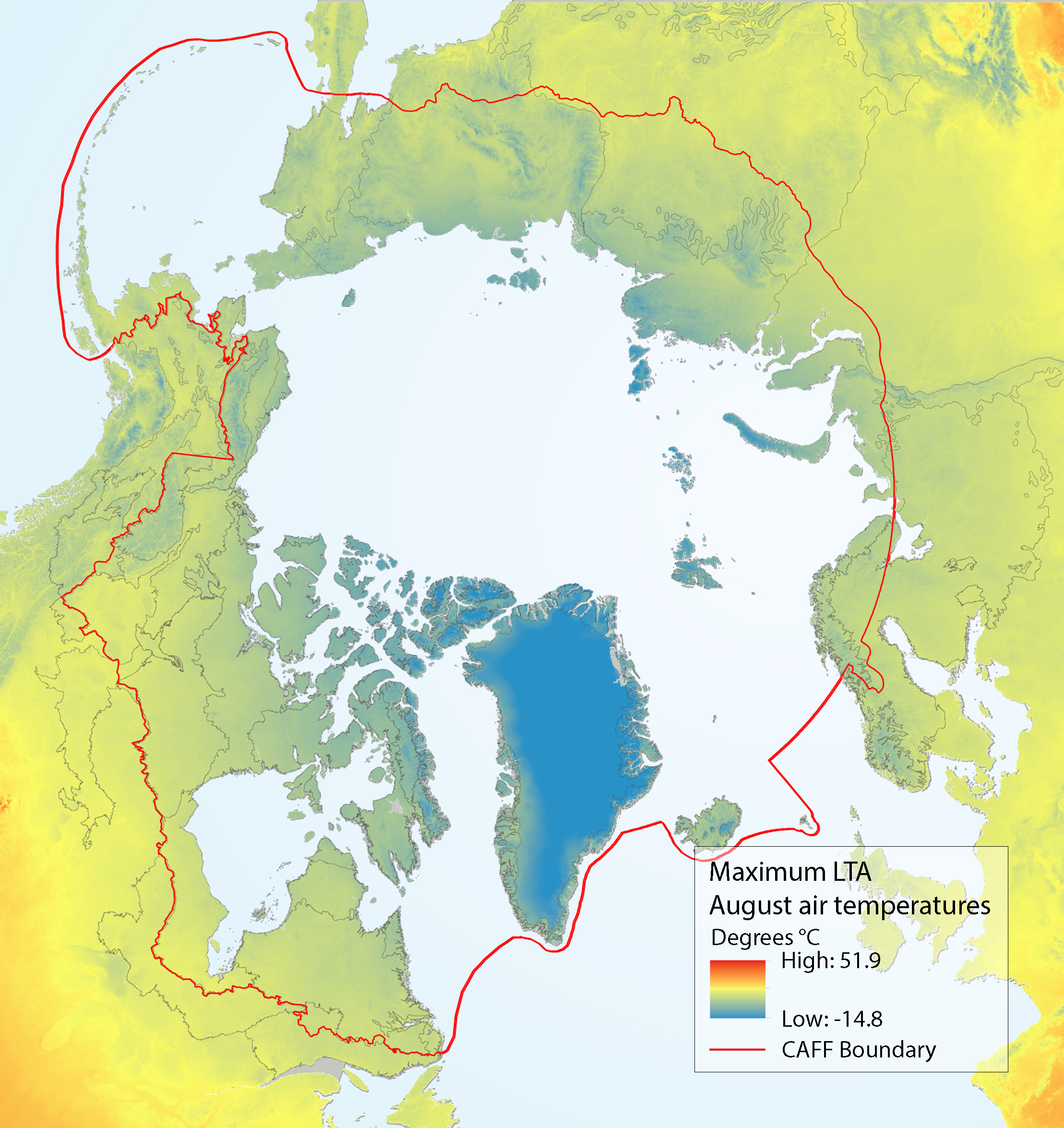
Maximum LTA (long-term average) August air temperatures for the circumpolar region, with ecoregions used in the analysis of the SAFBR outlined in black. Source for temperature layer: Fick and Hijmans (2017). State of the Arctic Freshwater Biodiversity Report - Chapter 5 - Page 89 - Figure 5-5
-
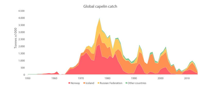
Global catches of all capelin species from 1950 to 2011 (FAO 2015). STATE OF THE ARCTIC MARINE BIODIVERSITY REPORT - <a href="https://arcticbiodiversity.is/findings/marine-fishes" target="_blank">Chapter 3</a> - Page 119 - Figure 3.4.6
-
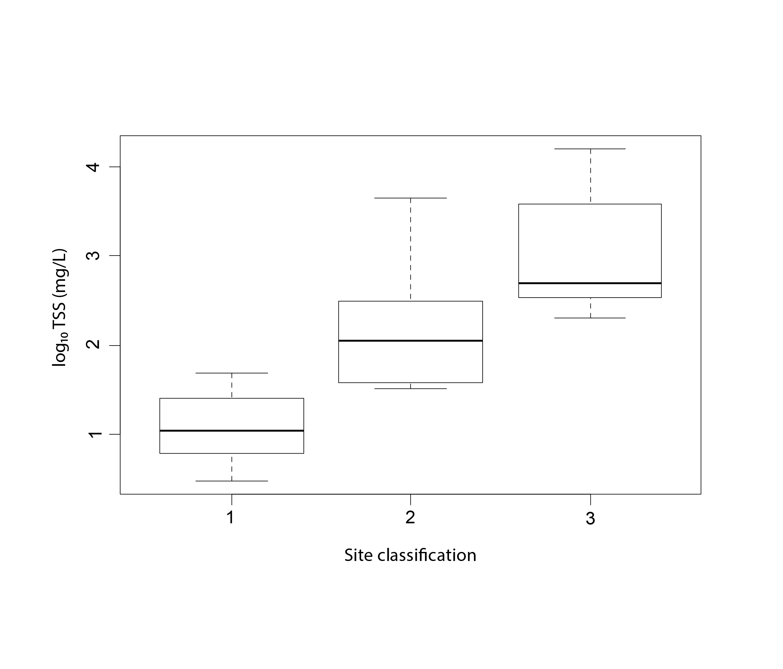
Figure 3-4 Effects of permafrost thaw slumping on Arctic rivers, including (upper) a photo of thaw slump outflow entering a stream on the Peel Plateau, Northwest Territories, Canada, and (lower) log10-transformed total suspended solids (TSS) in (1) undisturbed, (2) 1-2 disturbance, and (3) > 2 disturbance stream sites, with letters indicating significant differences in mean TSS among disturbance classifications Plot reproduced from Chin et al. (2016). State of the Arctic Freshwater Biodiversity Report - Chapter3 - Page 21 - Figure 3-4
-
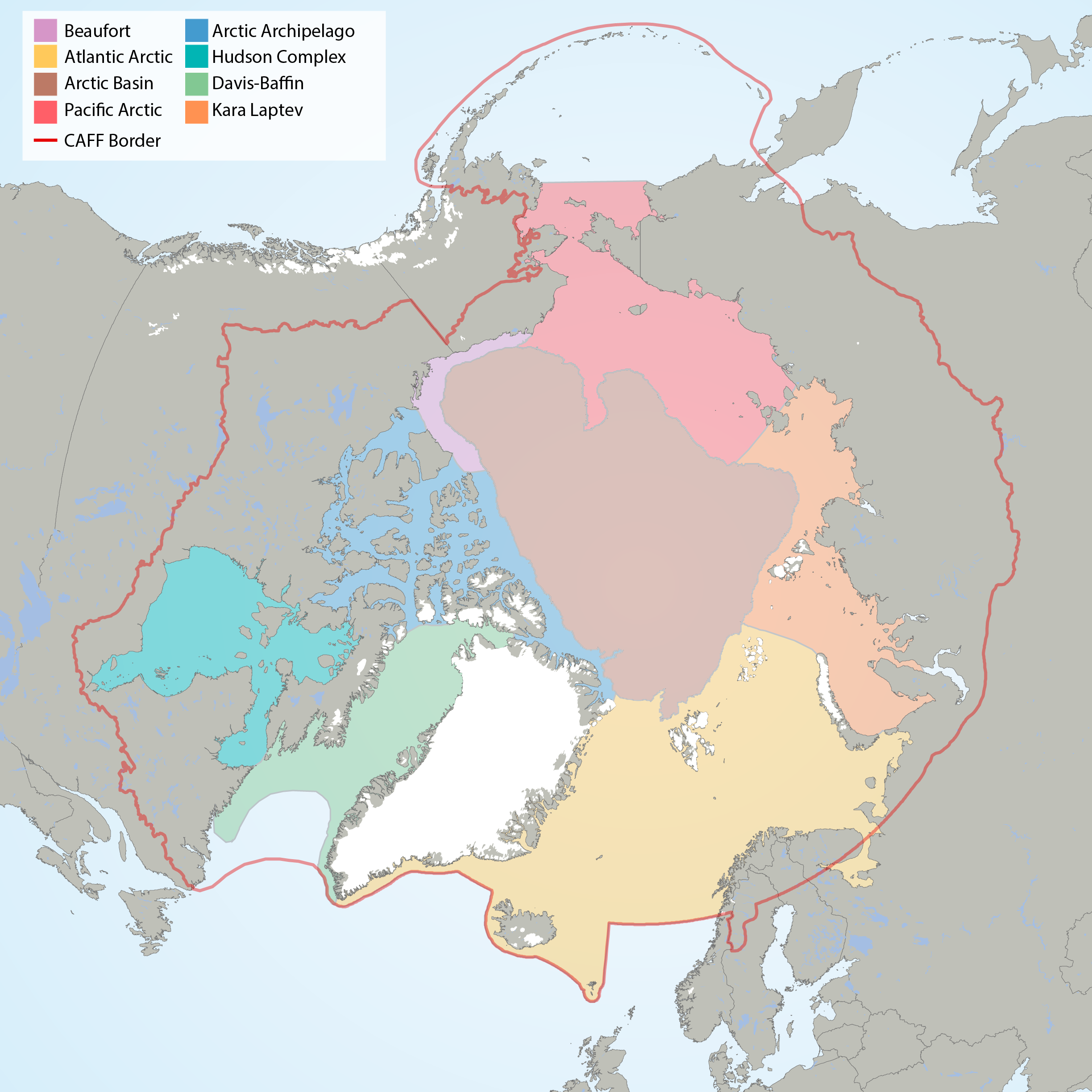
Arctic Marine Areas (AMAs) as defined in the CBMP Marine Plan. STATE OF THE ARCTIC MARINE BIODIVERSITY REPORT - <a href="https://arcticbiodiversity.is/marine" target="_blank">Chapter 1</a> - Page 15 - Figure 1.2