 CAFF - Arctic Biodiversity Data Service (ABDS)
oceans
Type of resources
Available actions
Topics
Keywords
Contact for the resource
Provided by
Years
Formats
Representation types
Update frequencies
status
Scale
-
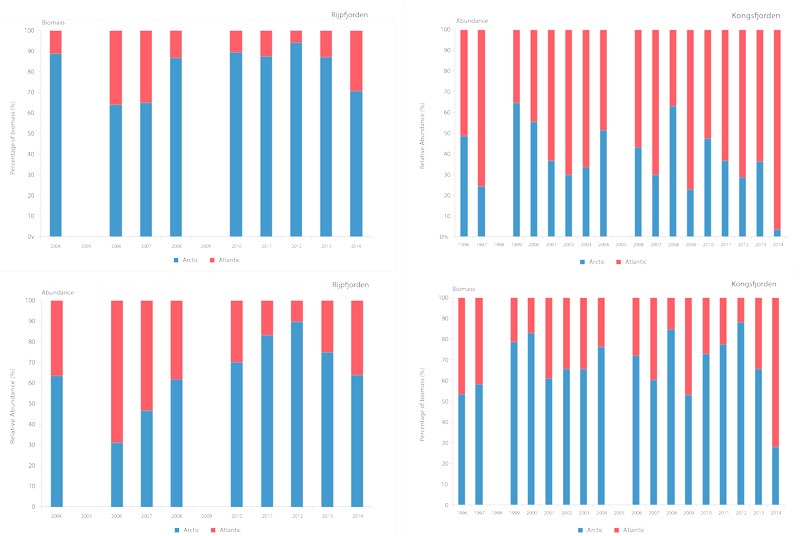
Time series of relative proportions of Arctic and Atlantic Calanus species in Kongsfjorden (top) and Rijpfjorden (bottom) (Source: MOSJ, Norwegian Polar Institute). STATE OF THE ARCTIC MARINE BIODIVERSITY REPORT - <a href="https://arcticbiodiversity.is/findings/plankton" target="_blank">Chapter 3</a> - Page 77 - Figure 3.2.8
-
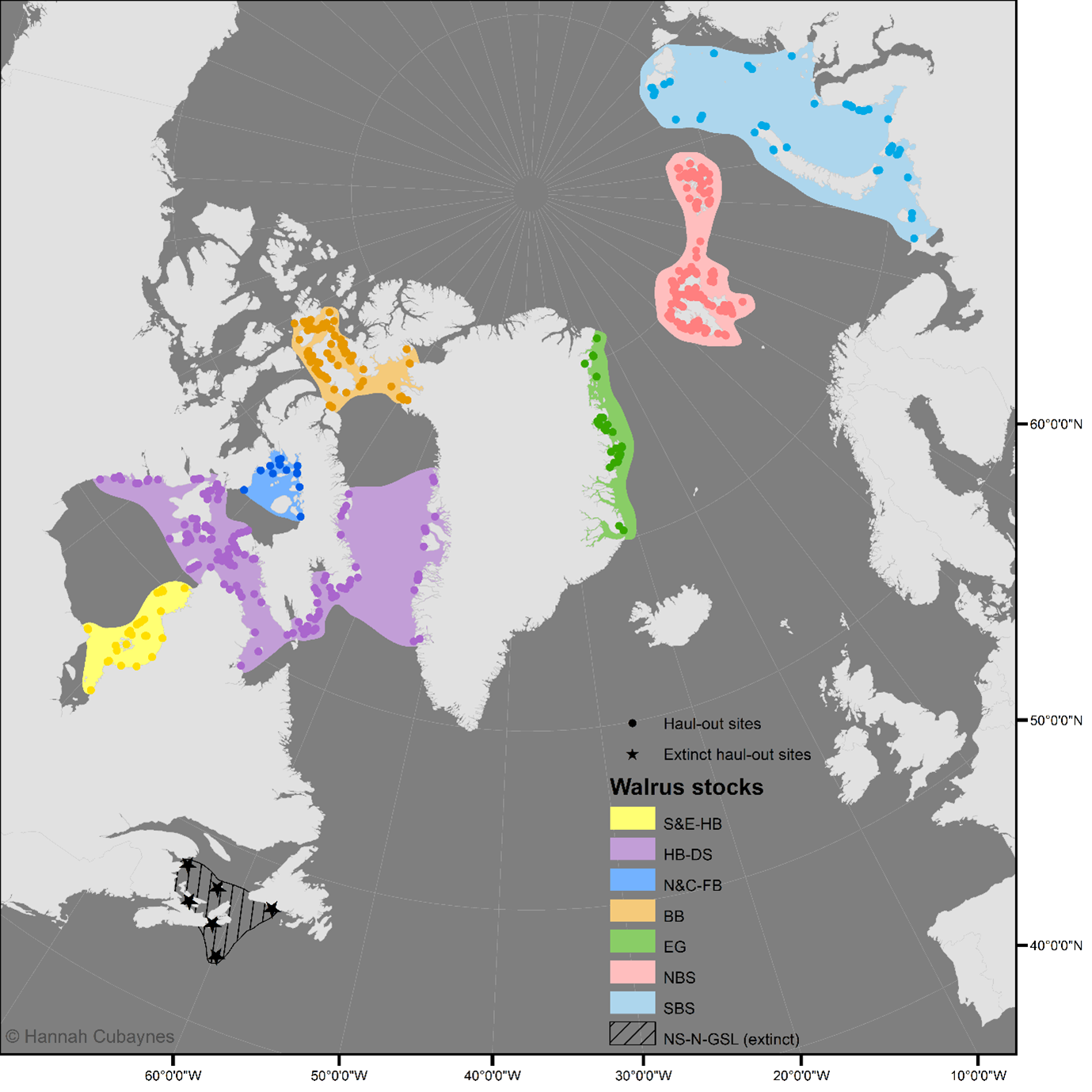
A dataset compiling all known terrestrial haul-out sites for the Atlantic walrus. The dataset comprises of the following documents: (1) the database in .csv format: walrus_haulout_database_Atlantic_caff_v4.csv; (2) the database in .shp format: walrus_haulout_database_Atlantic_caff_v4.shp; and (3) a user guidance document: user_guidance_atlantic_walrus_db.docx. The dataset will be updated annually. The latest update was 14th May 2025.
-
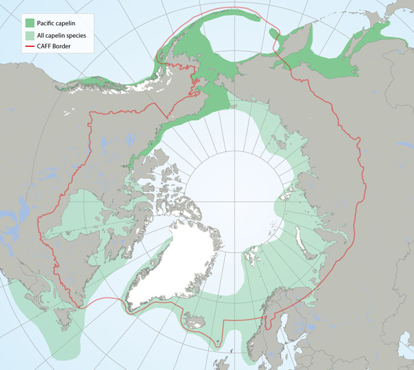
Distributions of all capelin species (light green) and Pacific capelin (Mallotus catervarius; dark green pattern) based on participation in research sampling, examination of museum voucher collections, the literature and molecular genetic analysis (Mecklenburg and Steinke 2015, Mecklenburg et al. 2016). Map shows the maximum distribution observed from point data and includes both common and rare locations STATE OF THE ARCTIC MARINE BIODIVERSITY REPORT - <a href="https://arcticbiodiversity.is/findings/marine-fishes" target="_blank">Chapter 3</a> - Page 117 - Figure 3.4.5
-
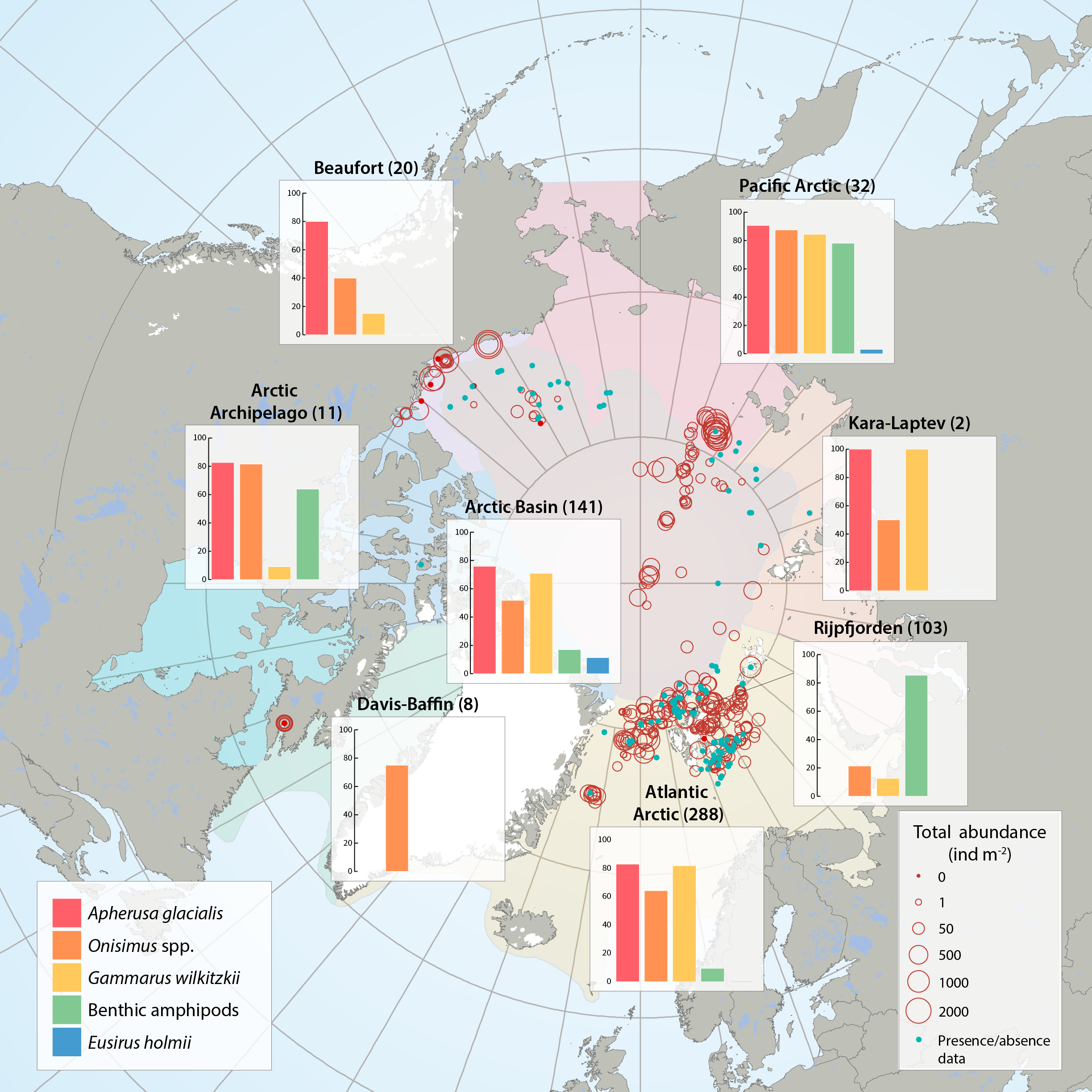
Sea ice amphipod (macrofauna) distribution and abundance across the Arctic aggregated from 47 sources between 1977 and 2012 by the CBMP Sea Ice Biota Expert Network. Bar graphs illustrate the frequency of occurrence (%) of amphipods in samples that contained at least one ice-associated amphipod. Red circles illustrate the total abundances of all ice-associated amphipods in quantitative samples (individuals m-2) at locations of sampling for each Arctic Marine Area (AMA). Number of sampling efforts for each region is given in parenthesis after region name. Blue dots represent samples where only presence/ absence data were available and where amphipods were present. STATE OF THE ARCTIC MARINE BIODIVERSITY REPORT - <a href="https://arcticbiodiversity.is/findings/sea-ice-biota" target="_blank">Chapter 3</a> - Page 44 - Figure 3.1.6 From the report draft: "This summary includes 47 data sources of under-ice amphipods published between 1977 and 2012. When available, we collected information on abundance or density (ind. m-2, or ind. m-3 that were converted to ind. m-2) and biomass (g m-2, wet weight). If abundance or biomass data were not available, we examined presence/relative abundance information. Frequency of occurrence was calculated for regions across the Arctic using integrated data for all available years."
-
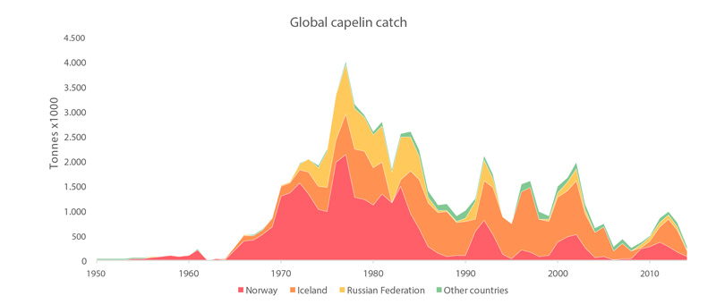
Global catches of all capelin species from 1950 to 2011 (FAO 2015). STATE OF THE ARCTIC MARINE BIODIVERSITY REPORT - <a href="https://arcticbiodiversity.is/findings/marine-fishes" target="_blank">Chapter 3</a> - Page 119 - Figure 3.4.6
-

Interannual differences in taxonomic composition of phytoplankton during summer in a) Kongsfjorden and b) Rijpfjorden (Source: MOSJ, Norwegian Polar Institute). STATE OF THE ARCTIC MARINE BIODIVERSITY REPORT - <a href="https://arcticbiodiversity.is/findings/plankton" target="_blank">Chapter 3</a> - Page 74 - Figure 3.2.5
-
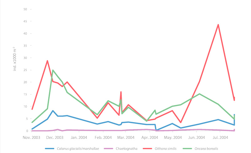
Seasonal time series of the major zooplankton in Franklin Bay, Canada STATE OF THE ARCTIC MARINE BIODIVERSITY REPORT - <a href="https://arcticbiodiversity.is/findings/plankton" target="_blank">Chapter 3</a> - Page 78 - Figure 3.2.9 Mesozooplankton abundance, integrated from 10 m above the seafloor to the surface (ind m-2), in Franklin Bay during the CASES 2003-04 overwintering expedition. Most of the sampling was done at the overwintering station and a few stations were close to this site in autumn 2003 and summer 2004.
-
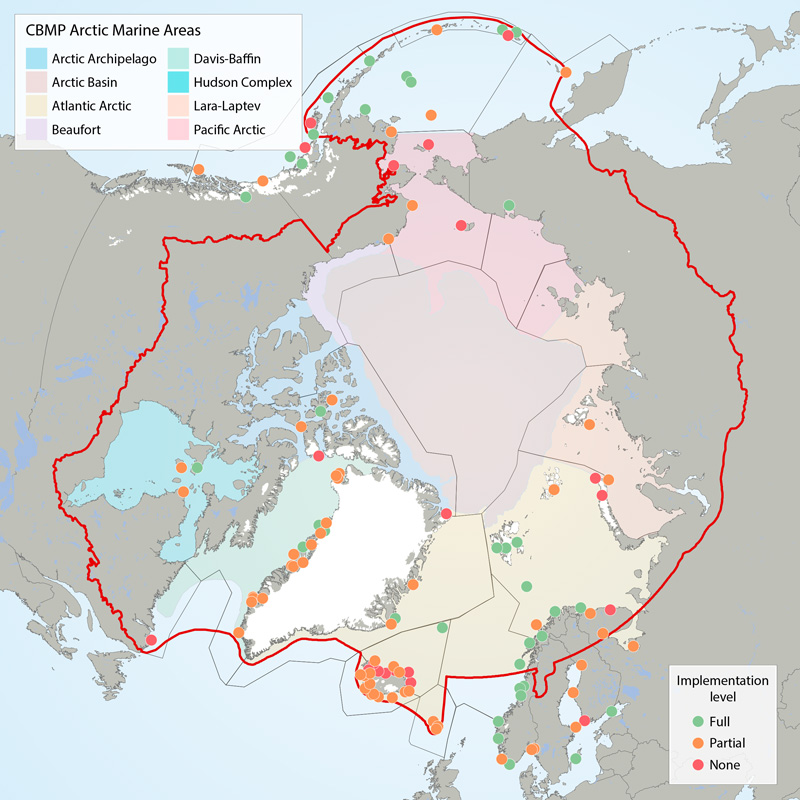
Boundaries of the 22 ecoregions (grey lines) as defined in the CSMP (Irons et al. 2015) and the Arctic Marine Areas (colored polygons with names in legend). Filled circles show locations of seabird colony sites recommended for monitoring (‘key sites’). The current level of monitoring plan implementation are green = fully implemented, amber = partially implemented, red = not implemented. The CSMP provides implementation maps for each forage guild. STATE OF THE ARCTIC MARINE BIODIVERSITY REPORT - <a href="https://arcticbiodiversity.is/findings/seabirds" target="_blank">Chapter 3</a> - Page 132 - Figure 3.5.1 This graphic displays the status of seabird monitoring at key sites in CBMP areas across the Arctic.
-
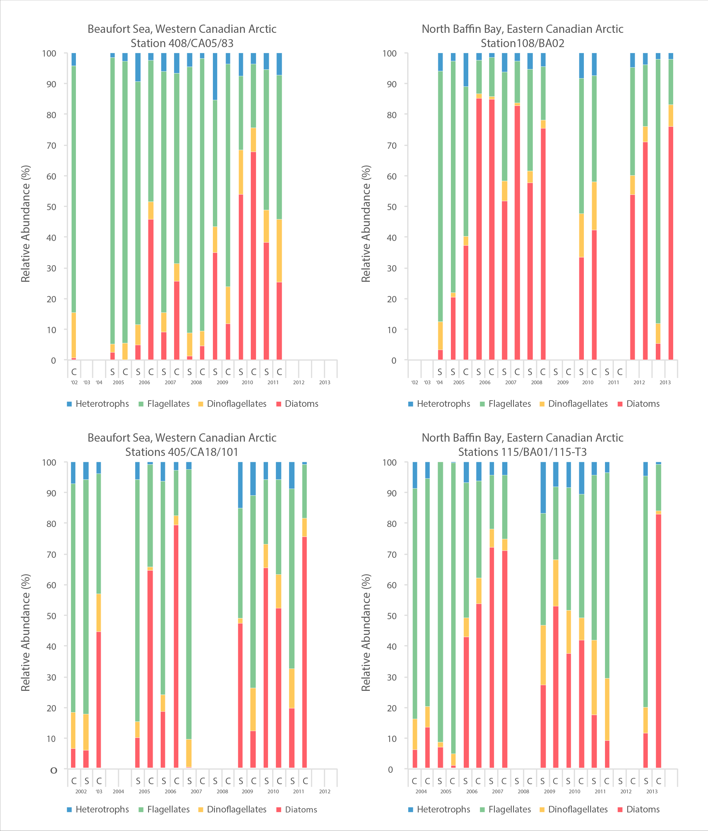
A time series of cell abundances, as determined by microscopy, of major phytoplankton groups from 2002-2013 for four sites, two in an east-west transect in Amundsen Gulf, Beaufort Sea and two in an east-west transect in northern Baffin Bay. STATE OF THE ARCTIC MARINE BIODIVERSITY REPORT - <a href="https://arcticbiodiversity.is/findings/plankton" target="_blank">Chapter 3</a> - Page 73 - Figure 3.2.4 A time series of cell abundances, as determined by microscopy, of major phytoplankton groups from 2002-2013 for four sites, 2 in the Beaufort Sea and 2 in northern Baffin Bay. Cell abundances are given as cells per liter. On most sampling dates, there is data from surface water and from the subsurface chlorophyll maximum (Cmax in the spreadsheet). Some additional information is included in the column headings, such as the percent of light at the sample depth; however, this should not be included in the figure. You may or may not want to include a map element in this figure, and rough coordinates of the sampling sites are included. The second sheet of the excel file presents the same data but at a finer scale of taxonomic resolution. It is the first sheet that should be used.
-
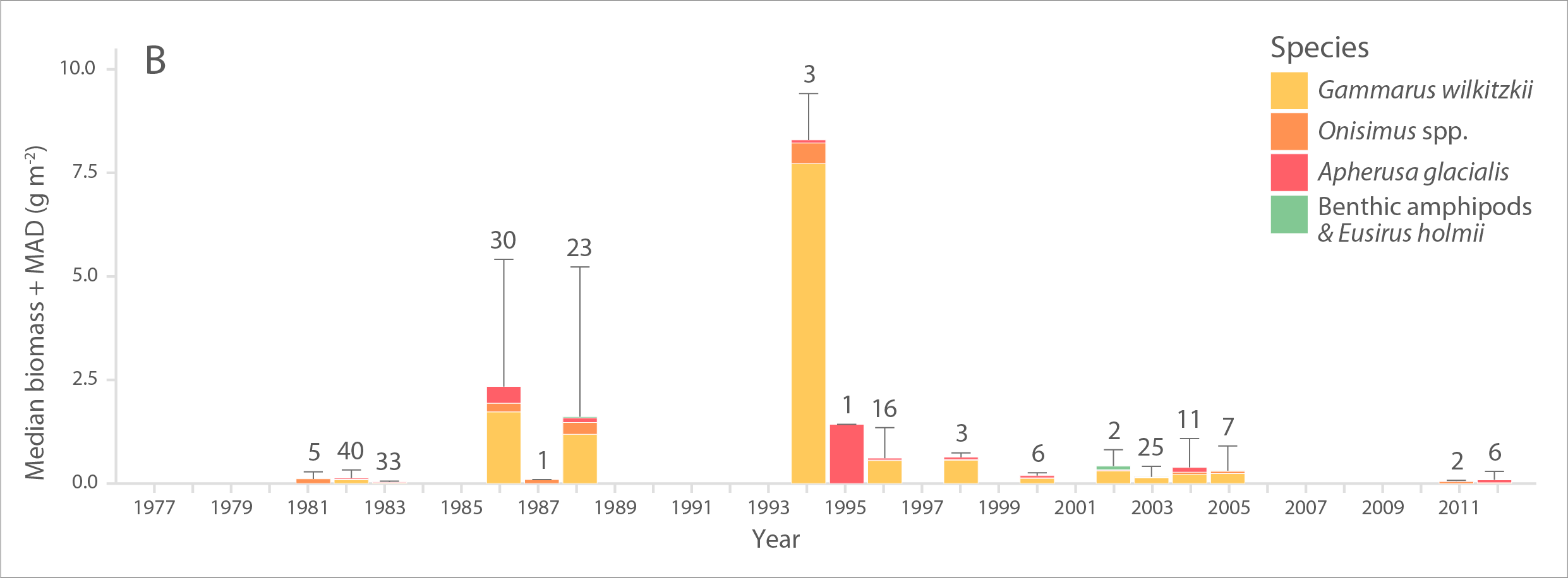
Multi-decadal time series of A) abundance (individuals m-2) and B) biomass (g wet weight m-2) of ice amphipods from 1977 to 2012 across the Arctic. Bars and error bars indicate median and median absolute deviation (MAD) values for each year, respectively. Numbers above bars represent number of sampling efforts (n). Modified from Hop et al. (2013). STATE OF THE ARCTIC MARINE BIODIVERSITY REPORT - <a href="https://arcticbiodiversity.is/findings/sea-ice-biota" target="_blank">Chapter 3</a> - Page 45 - Figure 3.1.7 From the report draft: "The only available time-series of sympagic biota is based on composite data of ice-amphipod abundance and biomass estimates from the 1980s to present across the Arctic, with most observations from the Svalbard and Fram Strait region (Hop et al. 2013). Samples were obtained by SCUBA divers who collected amphipods quantitatively with electrical suction pumps under the sea ice (Lønne & Gulliksen 1991a, b, Hop & Pavlova 2008)."