 CAFF - Arctic Biodiversity Data Service (ABDS)
oceans
Type of resources
Available actions
Topics
Keywords
Contact for the resource
Provided by
Years
Formats
Representation types
Update frequencies
status
Scale
-
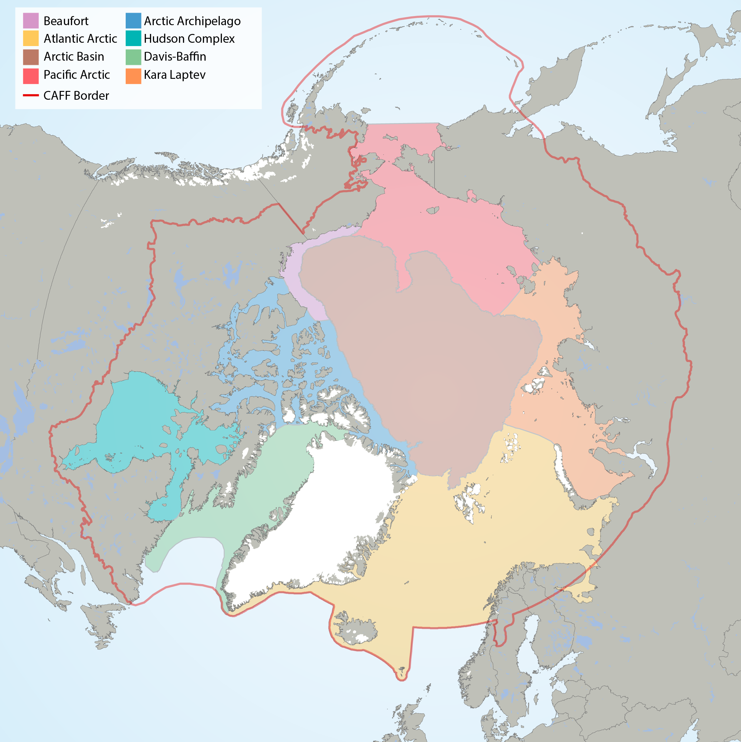
Arctic Marine Areas (AMAs) as defined in the CBMP Marine Plan. STATE OF THE ARCTIC MARINE BIODIVERSITY REPORT - <a href="https://arcticbiodiversity.is/marine" target="_blank">Chapter 1</a> - Page 15 - Figure 1.2
-
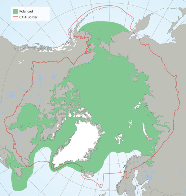
Distribution of polar cod (Boreogadus saida) based on participation in research sampling, examination of museum voucher collections and the literature (Mecklenburg et al. 2011, 2014, 2016; Mecklenburg and Steinke 2015). Map shows the maximum distribution observed from point data and includes both common and rare locations. STATE OF THE ARCTIC MARINE BIODIVERSITY REPORT - <a href="https://arcticbiodiversity.is/findings/marine-fishes" target="_blank">Chapter 3</a> - Page 114 - Figure 3.4.2
-
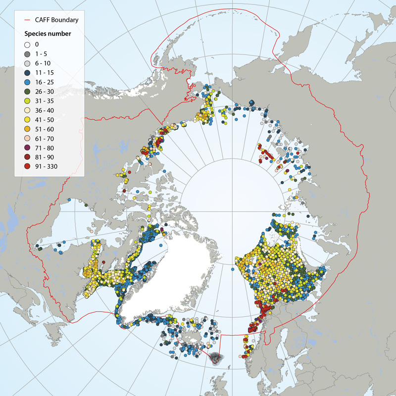
Number of megafauna species/taxa in the Arctic (7,322 stations in total), based on recent trawl investigations. Stations with highest species/taxon number are sorted to the top, meaning that dense concentrations of stations (e.g. Eastern Canada, Barents Sea), with low species numbers are hidden behind stations with higher species numbers. Also note that species numbers are somewhat biased by differing taxonomic resolution between studies. Data from: Icelandic Institute of Natural History, Iceland; Marine Research Institute, Iceland; University of Alaska, Fairbanks, U.S.; Greenland Institute of Natural Resources, Greenland; Zoological Institute of the Russian Academy of Sciences, St. Petersburg, Russia; Université du Québec à Rimouski, Canada; Fisheries and Oceans Canada; Institute of Marine Research, Norway; and Polar Research Institute of Marine Fisheries and Oceanography, Murmansk, Russia. STATE OF THE ARCTIC MARINE BIODIVERSITY REPORT - <a href="https://arcticbiodiversity.is/findings/benthos" target="_blank">Chapter 3</a> - Page 91 - Box figure 3.3.2 Several regions of the Pan Arctic have been sampled with trawl. Even though the trawl configurations and the taxonomic level are different from area to area, we choose to consider the taxonomic richness as relatively comparative.
-
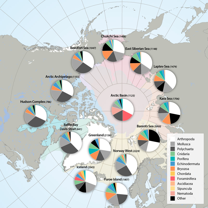
Arthropods (e.g., shrimps, crabs, sea spiders, amphipods, isopods) dominate taxon numbers in all Arctic regions, followed by polychaetes (e.g., bristle worms) and mollusks (e.g., gastropods, bivalves). Other taxon groups are diverse in some regions, such as bryozoans in the Kara Sea, cnidarians in the Atlantic Arctic, and foraminiferans in the Arctic deep-sea basins. This pattern is biased, however, by the meiofauna inclusion for the Arctic Basin (macro- and meiofauna size ranges overlap substantially in deep-sea fauna, so nematodes and foraminiferans are included) and the influence of a lack of specialists for some difficult taxonomic groups. STATE OF THE ARCTIC MARINE BIODIVERSITY REPORT - <a href="https://arcticbiodiversity.is/findings/benthos" target="_blank">Chapter 3</a> - Page 89 - Box figure 3.3.1 Each region of the Pan Arctic has been sampled with a set of different sampling gears, including grab, sledge and trawl, while other areas has only been sampled with grab. Here is the complete species/taxa number and the % distribution of species/taxa in main phyla, per region of the Pan Arctic.
-
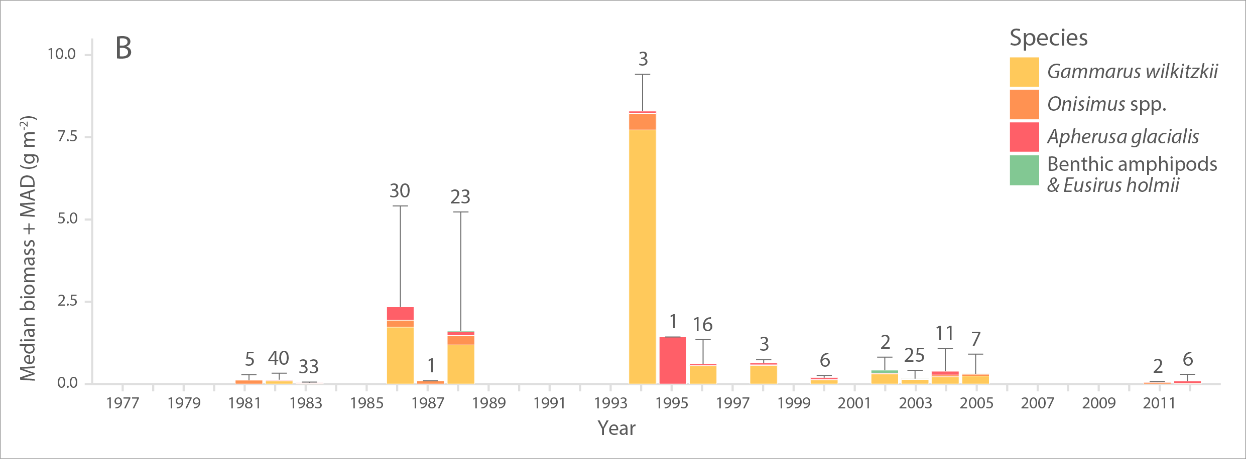
Multi-decadal time series of A) abundance (individuals m-2) and B) biomass (g wet weight m-2) of ice amphipods from 1977 to 2012 across the Arctic. Bars and error bars indicate median and median absolute deviation (MAD) values for each year, respectively. Numbers above bars represent number of sampling efforts (n). Modified from Hop et al. (2013). STATE OF THE ARCTIC MARINE BIODIVERSITY REPORT - <a href="https://arcticbiodiversity.is/findings/sea-ice-biota" target="_blank">Chapter 3</a> - Page 45 - Figure 3.1.7 From the report draft: "The only available time-series of sympagic biota is based on composite data of ice-amphipod abundance and biomass estimates from the 1980s to present across the Arctic, with most observations from the Svalbard and Fram Strait region (Hop et al. 2013). Samples were obtained by SCUBA divers who collected amphipods quantitatively with electrical suction pumps under the sea ice (Lønne & Gulliksen 1991a, b, Hop & Pavlova 2008)."
-
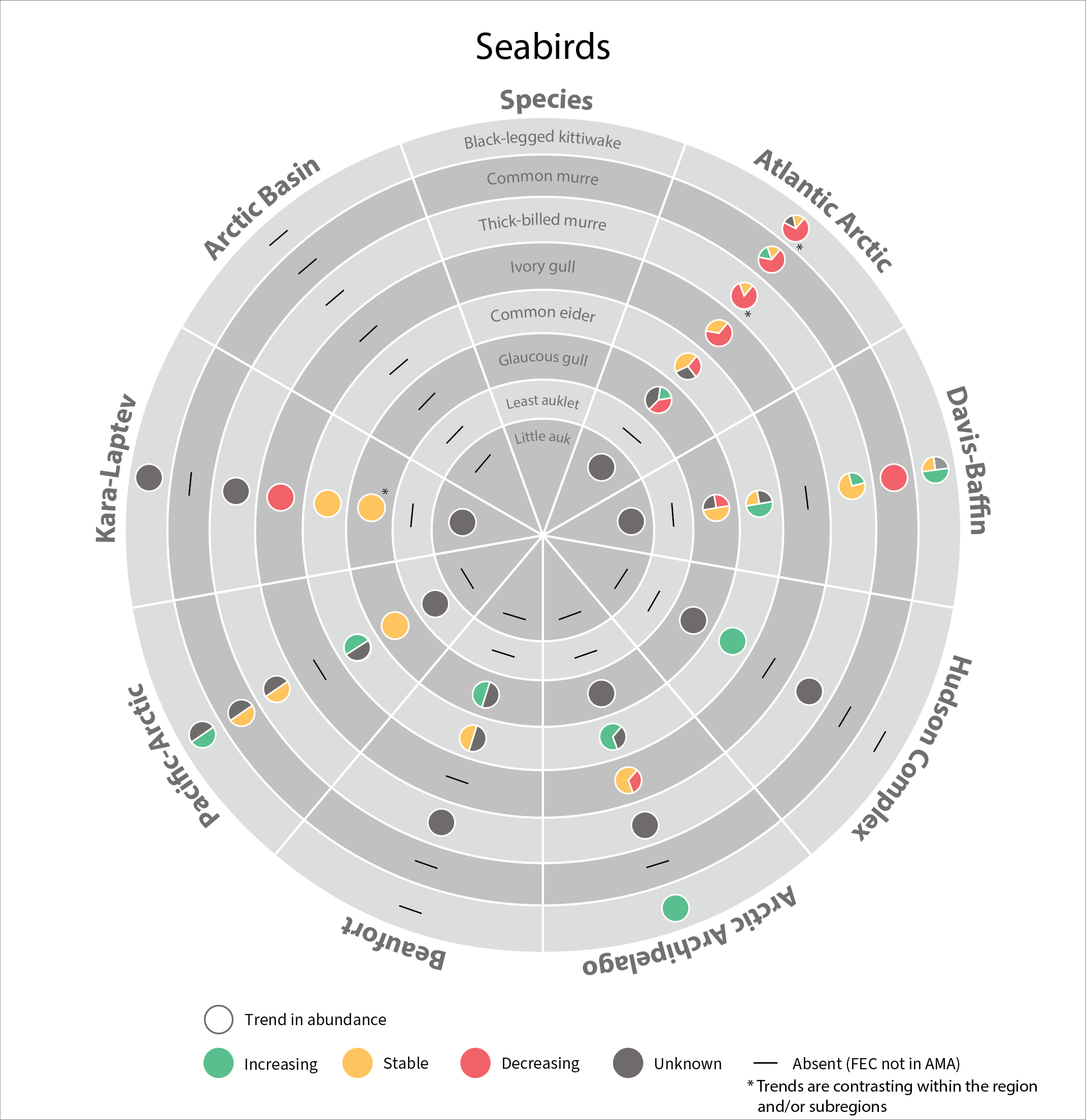
In 2017, the SAMBR synthesized data about biodiversity in Arctic marine ecosystems around the circumpolar Arctic. SAMBR highlighted observed changes and relevant monitoring gaps using data compiled through 2015. In 2021 an update was provided on the status of seabirds in circumpolar Arctic using data from 2016–2019. Most changes reflect access to improved population estimates, orimproved data for monitoring trends,independent of recognized trends in population size.
-
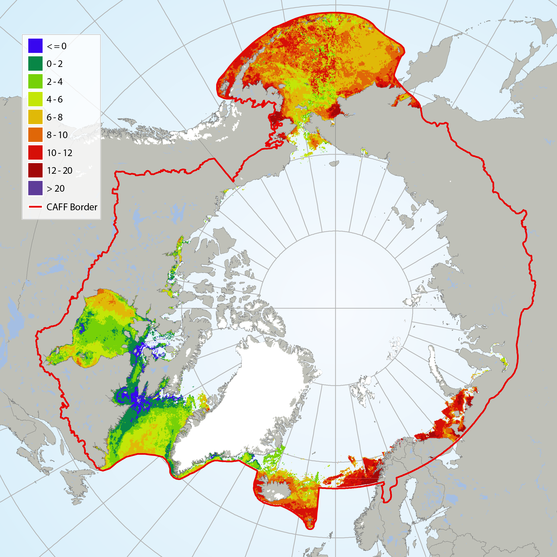
It has not been possible to identify available trend data for Arctic Ocean sea surface temperatures because there is not enough data to calculate reliable long-term trends for much of the Arctic marine environment (IPCC 2013, NOAA 2015). Here, sea surface temperature for July 2015 is shown from CAFF’s Land Cover Change Index. MODIS Sea Surface Temperature (SST) provided a four-kilometre spatial resolution monthly composite snapshot made from night-time measurements from the NASA Aqua Satellite. The night-time measurements are used to collect a consistent temperature measurement that is unaffected by the warming of the top layer of water by the sun. STATE OF THE ARCTIC MARINE BIODIVERSITY REPORT - <a href="https://arcticbiodiversity.is/marine" target="_blank">Chapter 2</a> - Page 25 - Figure 2.3
-
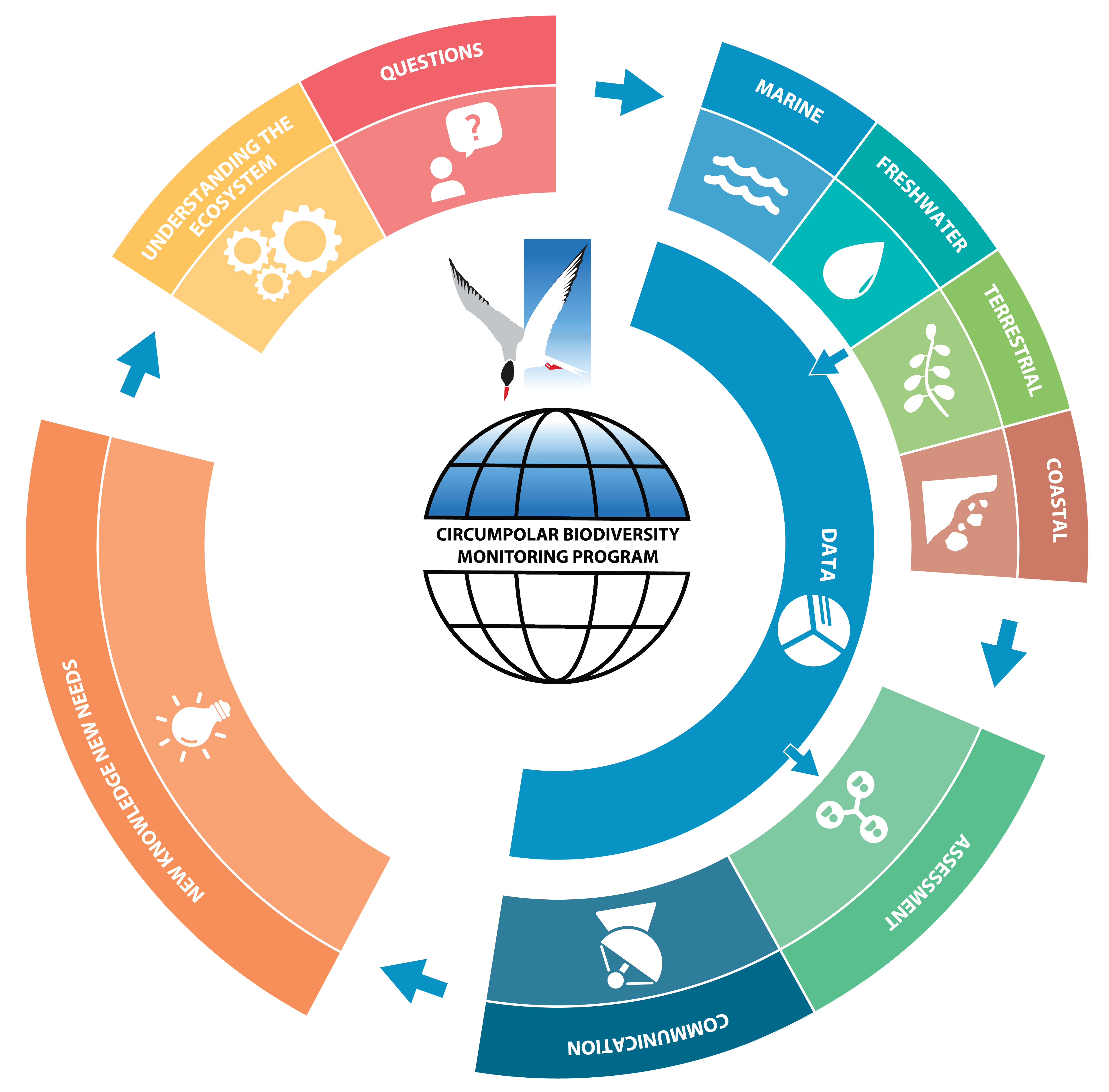
Workflow of the Circumpolar Biodiversity Monitoring Program (CBMP). STATE OF THE ARCTIC MARINE BIODIVERSITY REPORT - <a href="https://arcticbiodiversity.is/marine" target="_blank">Chapter 1</a> - Page 13 - Figure 1.1
-
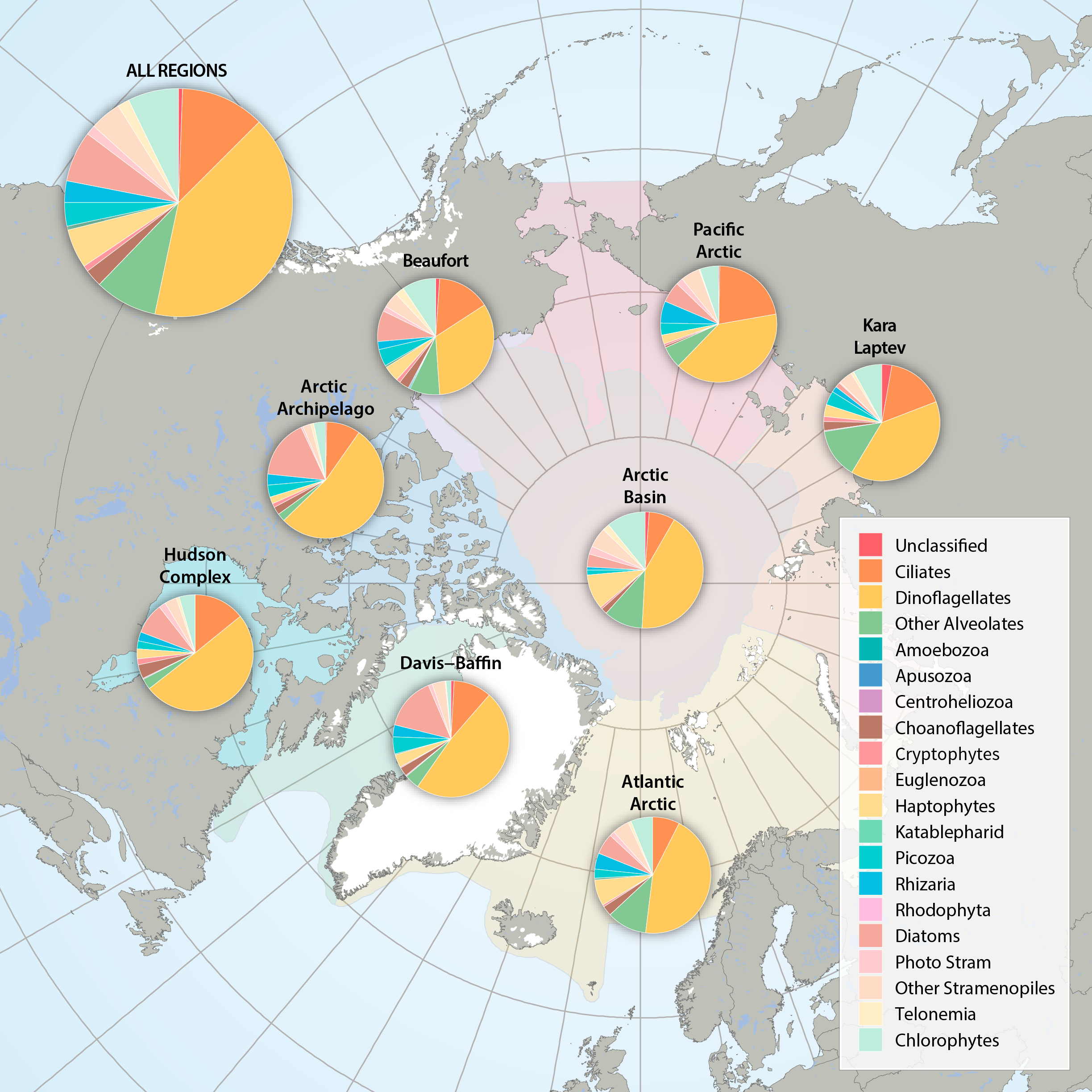
Figure 3.2.2a: Relative abundance of major eukaryote taxonomic groups found by high throughput sequencing of the small-subunit (18S) rRNA gene across Arctic Marine Areas. Figure 3.2.2b: Relative abundance of major eukaryote functional groups found by microscopy in the Arctic Marine Areas. STATE OF THE ARCTIC MARINE BIODIVERSITY REPORT - <a href="https://arcticbiodiversity.is/findings/plankton" target="_blank">Chapter 3</a> - Page 70 - Figures 3.2.2a and 3.2.2b
-
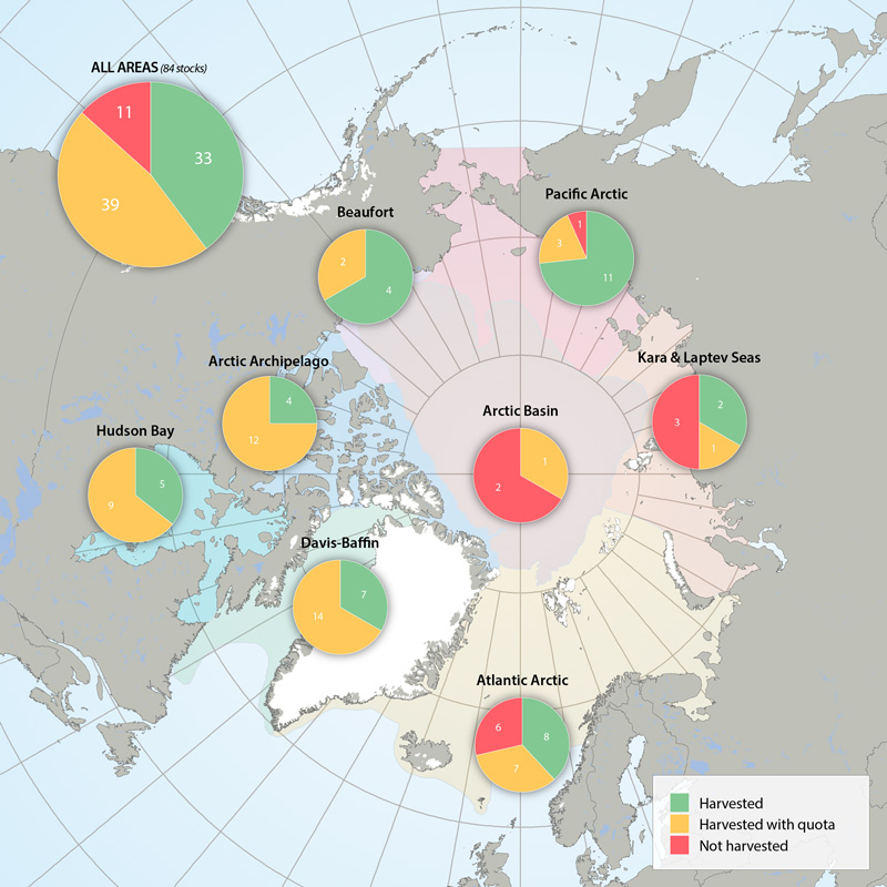
Harvest marine mammal Focal Ecosystem Component stocks in Arctic Marine Areas. Harvested without quotas, with quotas or not harvested. STATE OF THE ARCTIC MARINE BIODIVERSITY REPORT - <a href="https://arcticbiodiversity.is/findings/marine-mammals" target="_blank">Chapter 3</a> - Page 158 - Figure 3.6.4