 CAFF - Arctic Biodiversity Data Service (ABDS)
dataset
Type of resources
Available actions
Topics
Keywords
Contact for the resource
Provided by
Years
Formats
Representation types
Update frequencies
status
Scale
-
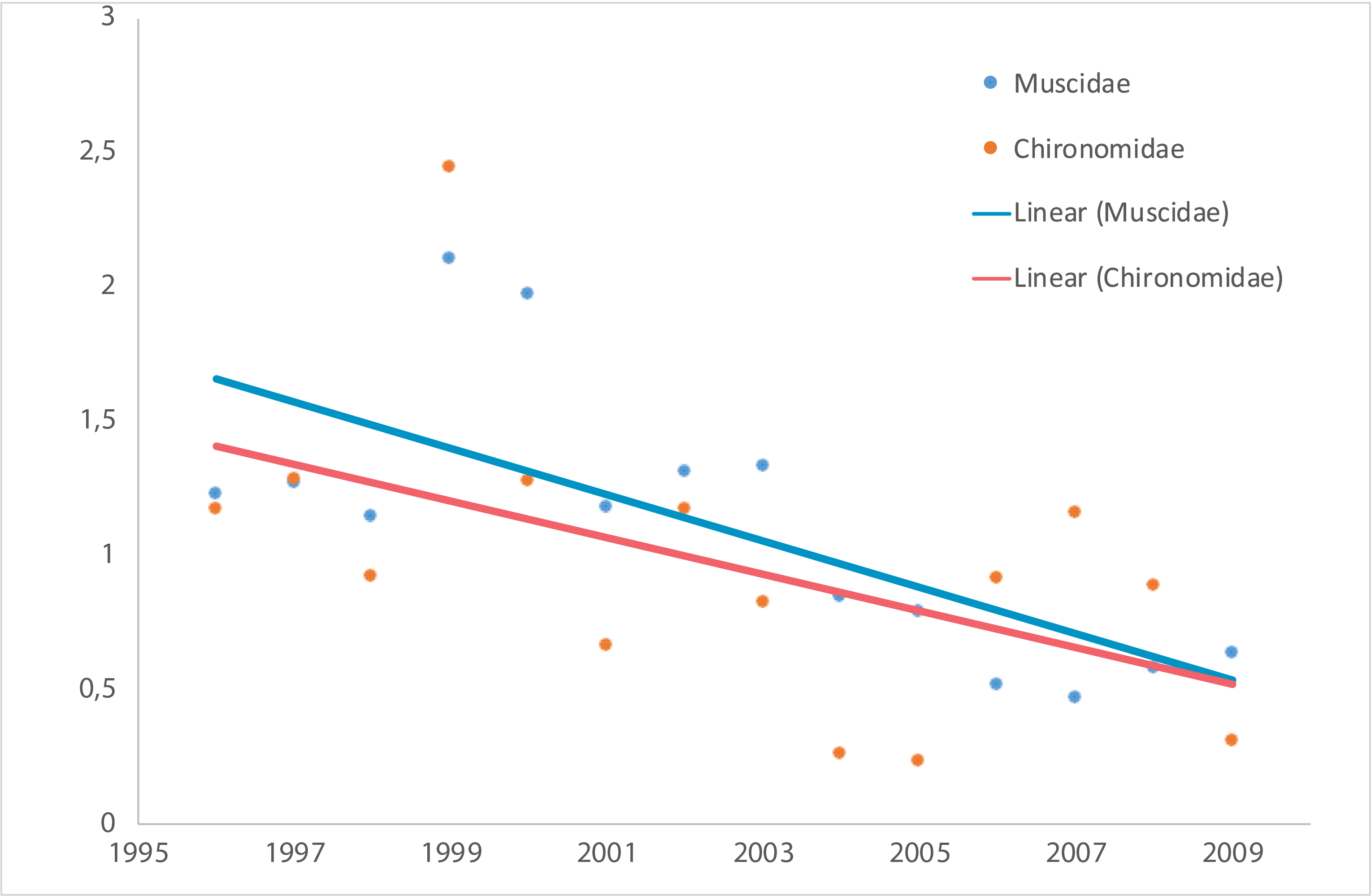
Temporal trends of arthropod abundance, 1996–2009. Estimated by the number of individuals caught per trap per day during the season from four different pitfall trap plots, each consisting of eight (1996–2006) or four (2007–2009) traps. Modified from Høye et al. 2013. STATE OF THE ARCTIC TERRESTRIAL BIODIVERSITY REPORT - Chapter 3 - Page 41 - Figure 3.16
-
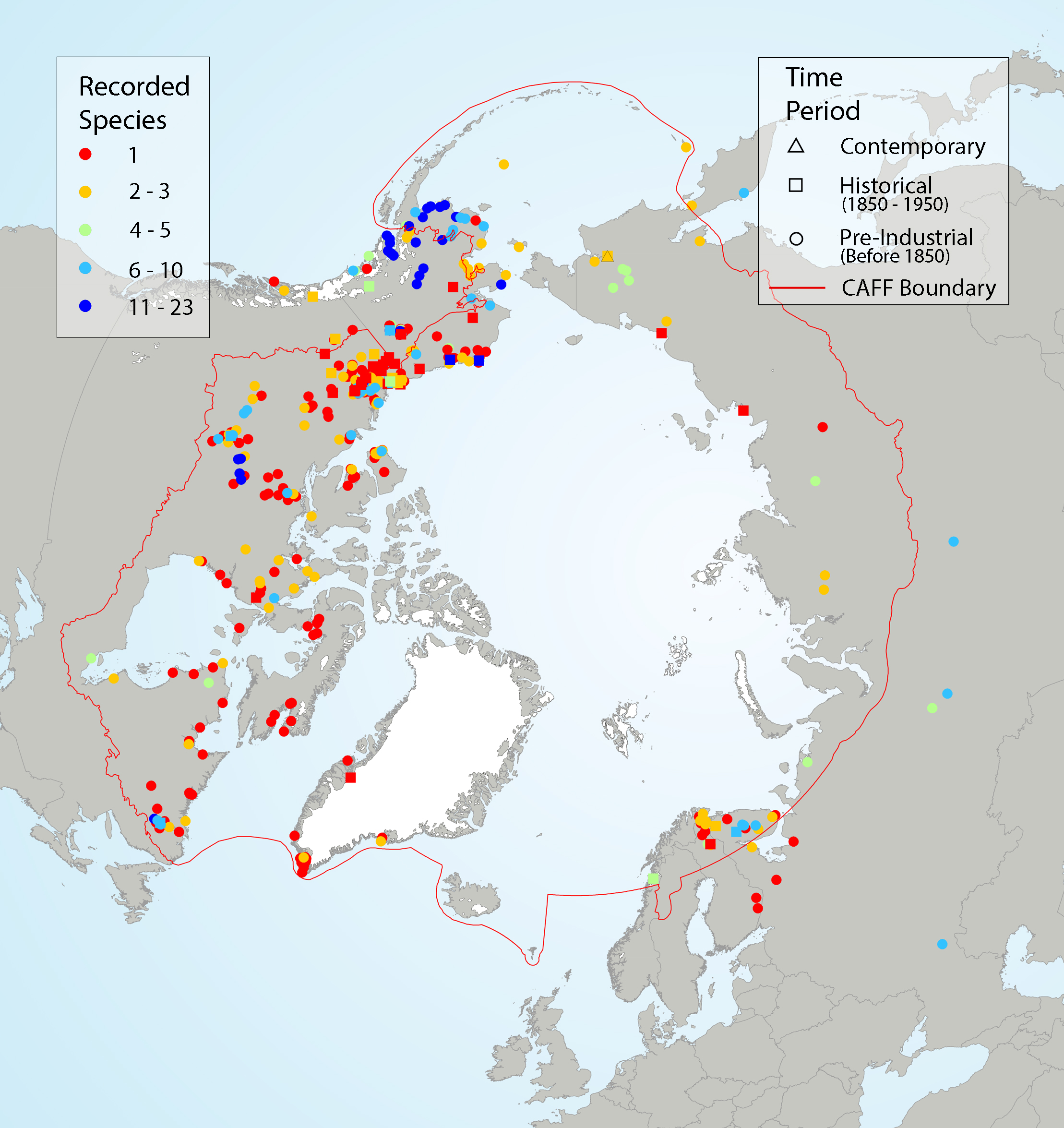
Fish species observations from Traditional Knowledge (TK ) literature, plotted in the approximate geographic location of observed record, with symbol colour indicating the number of fish species recorded and shape indicating the approximate time period of observation. Results are from a systematic literature search of TK sources from Alaska, Canada, Greenland, Fennoscandia, and Russia. State of the Arctic Freshwater Biodiversity Report - Chapter 4 - Page 75- Figure 4-37
-
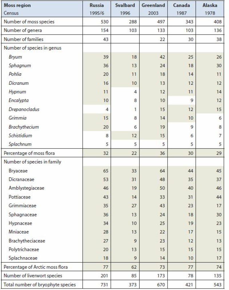
Arctic Biodiversity Assessment (ABA) 2013. Table 9.5. Species numbers of species-rich moss genera and families. Numbers highlighted in grey fields are used in calculating the percentage of the total moss flora. Listed are Splachnum, genera with at least 10 species and families with at least nine species. Conservation of Arctic Flora and Fauna, CAFF 2013 - Akureyri . Arctic Biodiversity Assessment. Status and Trends in Arctic biodiversity. - Plants(Chapter 9) page 333
-
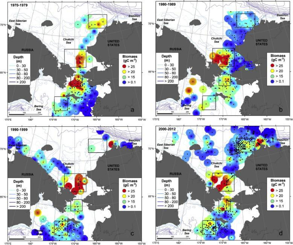
Benthic macro-infauna biomass in the northern Bering and Chukchi Seas from 1970 to 2012, displayed as decadal pattern Adapted from Grebmeier et al. (2015a) with permission from Elsevier. STATE OF THE ARCTIC MARINE BIODIVERSITY REPORT - <a href="https://arcticbiodiversity.is/findings/benthos" target="_blank">Chapter 3</a> - Page 98 - Figure 3.3.6 Cumulative scores of benthos drivers for each of the 8 CAFF-AMAs. The cumulative scores are taken from the last column of Table 3.3.1. The flower chart/plot helps to visualize the data.
-
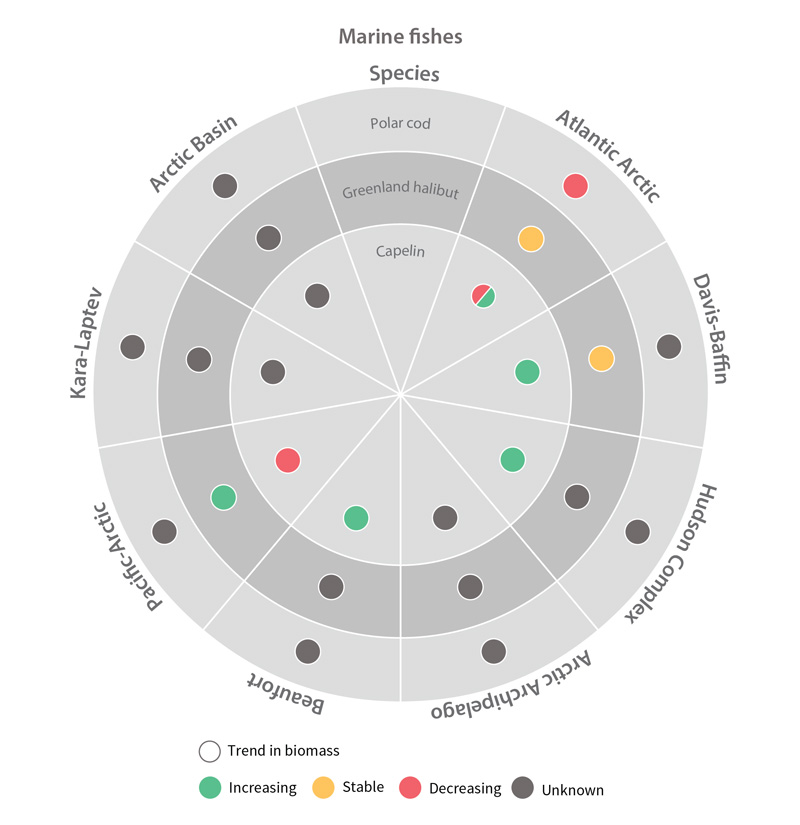
Trends in biomass of marine fish Focal Ecosystem Components across each Arctic Marine Area STATE OF THE ARCTIC MARINE BIODIVERSITY REPORT - Chapter 4 - Page 180 - Figure 4.4
-
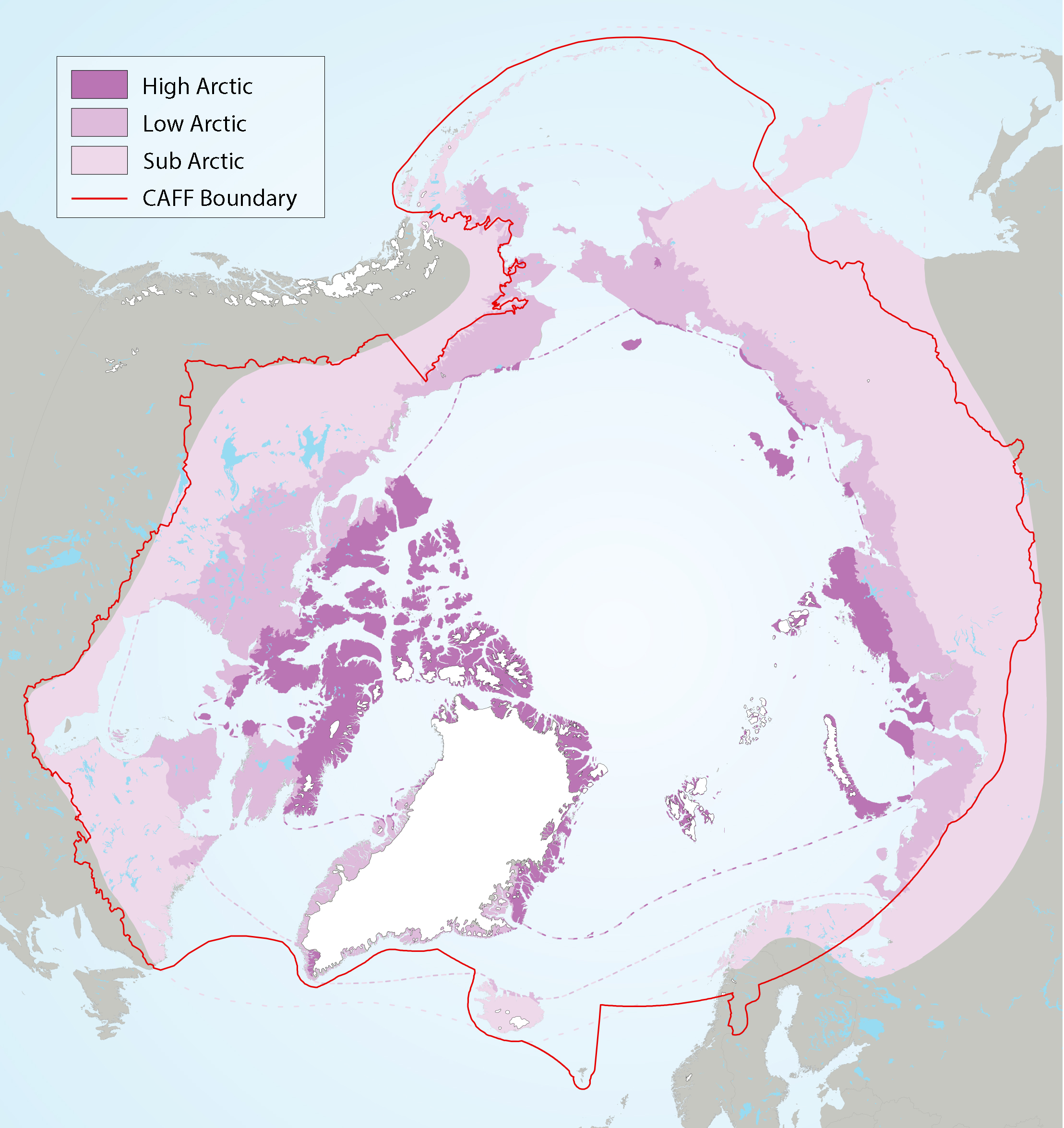
Figure 2-2 Arctic freshwater boundaries from the Arctic Council’s Arctic Biodiversity Assessment developed by CAFF, showing the three sub-regions of the Arctic, namely the high (dark purple), low (purple) and sub-Arctic (light purple)
-
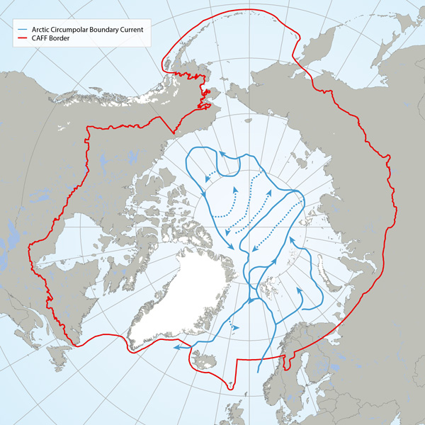
The Arctic Basin where suggested future long-term monitoring of trawl-megafauna should capture possible changes along the flow of the Arctic Circumpolar Boundary Current (Figure A, blue line) and the Arctic deep-water exchange (Figure b, green line). Adapted from Bluhm et al. (2015). STATE OF THE ARCTIC MARINE BIODIVERSITY REPORT - <a href="https://arcticbiodiversity.is/findings/benthos" target="_blank">Chapter 3</a> - Page 88 - Figure 3.3.1
-

Although the circumpolar countries endeavor to support monitoring programs that provide good coverage of Arctic and subarctic regions, this ideal is constrained by the high costs associated with repeated sampling of a large set of lakes and rivers in areas that often are very remote. Consequently, freshwater monitoring has sparse, spatial coverage in large parts of the Arctic, with only Fennoscandia and Iceland having extensive monitoring coverage of lakes and streams Figure 6-2 Current state of monitoring for river FECs in each Arctic country State of the Arctic Freshwater Biodiversity Report - Chapter 6 - Page 94 - Figure 6-2
-
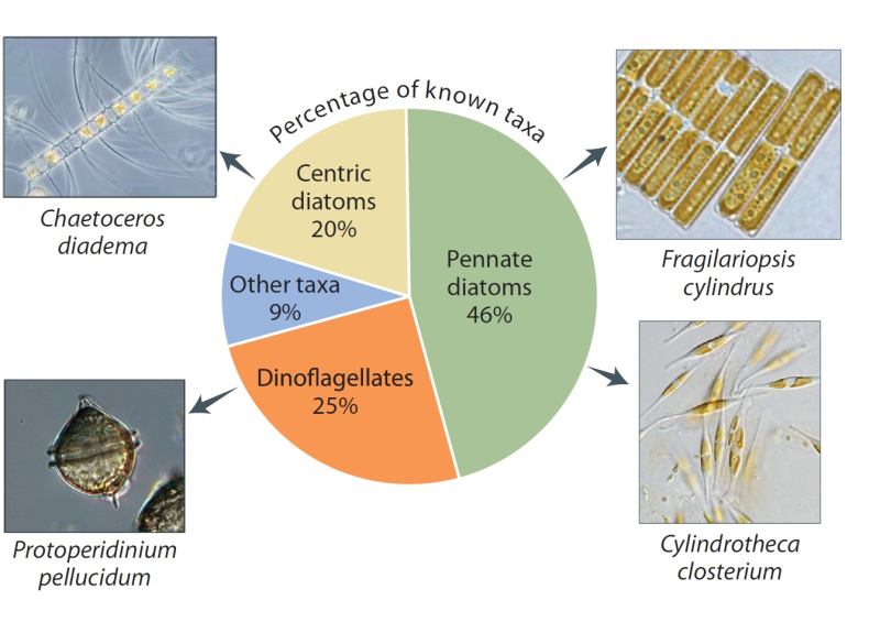
The number of species depends partly on what has been studied. Proportions vary somewhat around the Arctic, but diatoms and dinoflagellates are the most diverse groups everywhere. The greatest sampling effort has been in the Laptev Sea, Hudson Bay, and the Norwegian sector of the Barents Sea. Species shown are among the most commonly recorded. Published in the Life Linked to Ice released in 2013, page 26. Life Linked to Ice: A guide to sea-ice-associated biodiversity in this time of rapid change. CAFF Assessment Series No. 10. Conservation of Arctic Flora and Fauna, Iceland. ISBN: 978-9935-431-25-7.
-
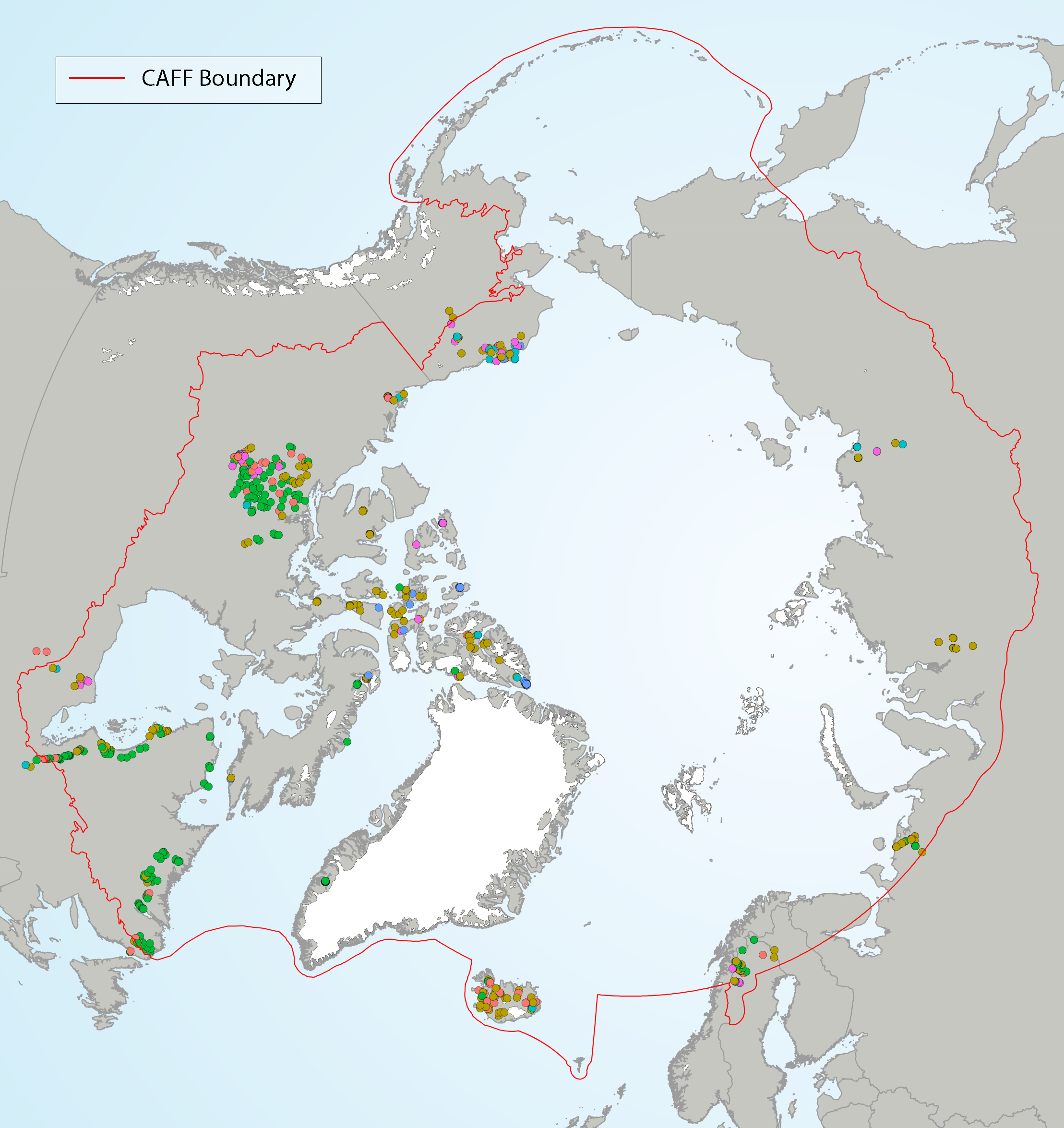
Figure 4 12 Diatom groups from Self Organizing Maps (SOMs) in lake top sediments, showing the geographical distribution of each group (with colors representing different SOM groups). State of the Arctic Freshwater Biodiversity Report - Chapter 4 - Page 39 - Figure 4-12