 CAFF - Arctic Biodiversity Data Service (ABDS)
Type of resources
Available actions
Topics
Keywords
Contact for the resource
Provided by
Years
Formats
Representation types
Update frequencies
status
Service types
Scale
-
The Seabird Information Network (SIN) developed by the Circumpolar Seabird expert group (<a href="http://caff.is/seabirds-cbird" target="_blank">CBird</a>) of the Conservation of Arctic Flora and Fauna (<a href="http://caff.is" target="_blank">CAFF</a>) working group of the Arctic Council focuses on the development of a data entry and analysis portal system allowing for circumpolar seabird colony information to be contributed, mapped, and shared by scientists and monitoring programs around the Arctic. - <a href="http://axiom.seabirds.net/maps/js/seabirds.php?app=circumpolar#z=2&ll=NaN,0.00000" target="_blank"> Circumpolar Seabird portal</a>
-
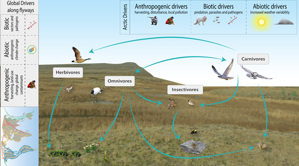
The CBMP–Terrestrial Plan identifies five FECs for monitoring terrestrial birds; herbivores, insectivores, carnivores, omnivores and piscivores. Due to their migratory nature, a wider range of drivers, from both within and outside the Arctic, affect birds and their associated FEC attributes compared to other terrestrial FECs. Figure 3-21 illustrates a conceptual model for Arctic terrestrial birds that includes examples of FECs and key drivers. STATE OF THE ARCTIC TERRESTRIAL BIODIVERSITY REPORT - Chapter 3 - Page 46 - Figure 3.21
-
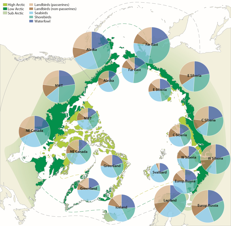
Figure 4.1. Avian biodiversity in different regions of the Arctic. Charts on the inner circle show species numbers of different bird groups in the high Arctic, on the outer circle in the low Arctic. The size of the charts is scaled to the number of species in each region, which ranges from 32 (Svalbard) to 117 (low Arctic Alaska). CAFF 2013. Arctic Biodiversity Assessment. Status and Trends in Arctic biodiversity. Conservation of Arctic Flora and Fauna, Akureyri - Birds (Chapter 4) page 145
-
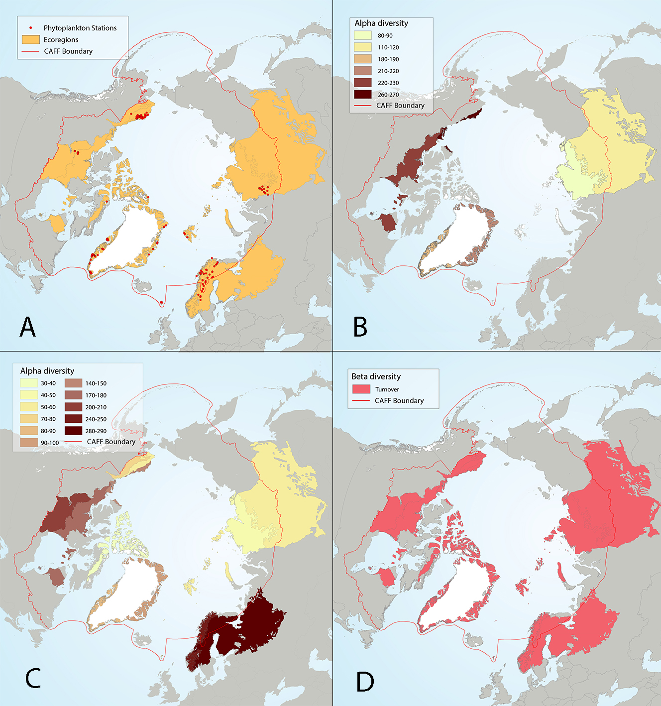
Figure 4 17 Results of circumpolar assessment of lake phytoplankton,(a) the location of phytoplankton stations, underlain by circumpolar ecoregions; (b) ecoregions with many phytoplankton stations, colored on the basis of alpha diversity rarefied to 35 stations; (c) all ecoregions with phytoplankton stations, colored on the basis of alpha diversity rarefied to 10 stations; (d) ecoregions with at least two stations in a hydrobasin, colored on the basis of the dominant component of beta diversity (species turnover, nestedness, approximately equal contribution, or no diversity) when averaged across hydrobasins in each ecoregion. State of the Arctic Freshwater Biodiversity Report - Chapter 4 - Page 56 - Figure 4-17
-
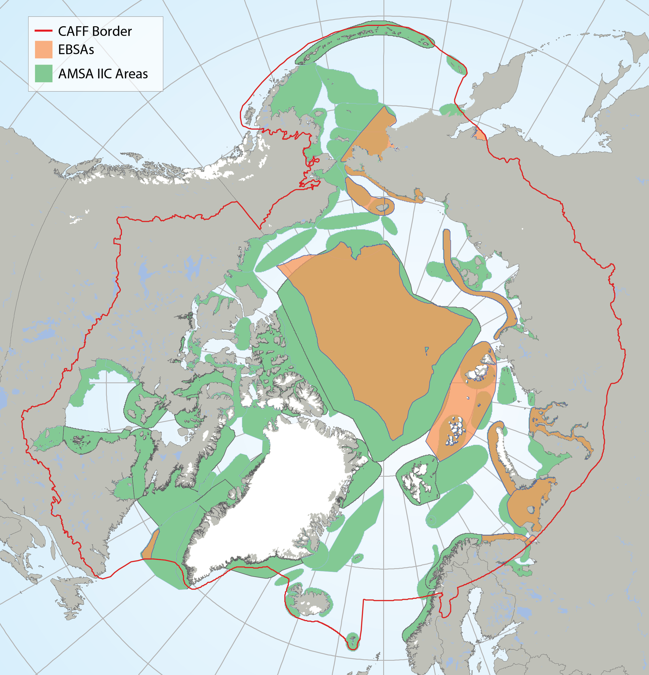
Arctic Ecologically and Biologically Significant Areas (EBSAs) and Arctic Marine Areas of Heightened Ecological and Cultural Significance as identified in the Arctic Marine Shipping Assessment (AMSA) IIC report. STATE OF THE ARCTIC MARINE BIODIVERSITY REPORT - <a href="https://arcticbiodiversity.is/marine" target="_blank">Chapter 1</a> - Page 16 - Box Figure 1.1
-
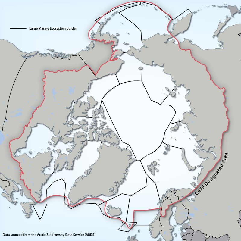
Large Marine Ecosystems (LMEs) are regions of ocean space encompassing coastal areas from river basins and estuaries to the seaward boundary of continental shelves and the seaward margins of coastal current systems. Fifty of them have been identified. They are relatively large regions (200 000 km2 or more) characterized by distinct bathymetry, hydrography, productivity and trophically dependent populations. The LME approach uses five modules: 1. productivity module considers the oceanic variability and its effect on the production of phyto and zooplankton 2. fish and fishery module concerned with the sustainability of individual species and the maintenance of biodiversity 3. pollution and ecosystem health module examines health indices, eutrophication, biotoxins, pathology and emerging diseases 4. socio-economic module integrates assessments of human forcing and the long-term sustainability and associated socio-economic benefits of various management measures, and 5. governance module involves adaptive management and stakeholder participation.” Source: http://www.fao.org/fishery/topic/3440/en Reference: Sherman, K. and Hempel, G. (Editors) 2009. The UNEP Large Marine Ecosystem Report: A perspective on changing conditions in LMEs of the world’s Regional Seas. UNEP Regional Seas Report and Studies No. 182. United Nations Environment Programme. Nairobi, Kenya. Data available from: http://lme.edc.uri.edu/ - LMEs of the world Updated shape file - 2014
-
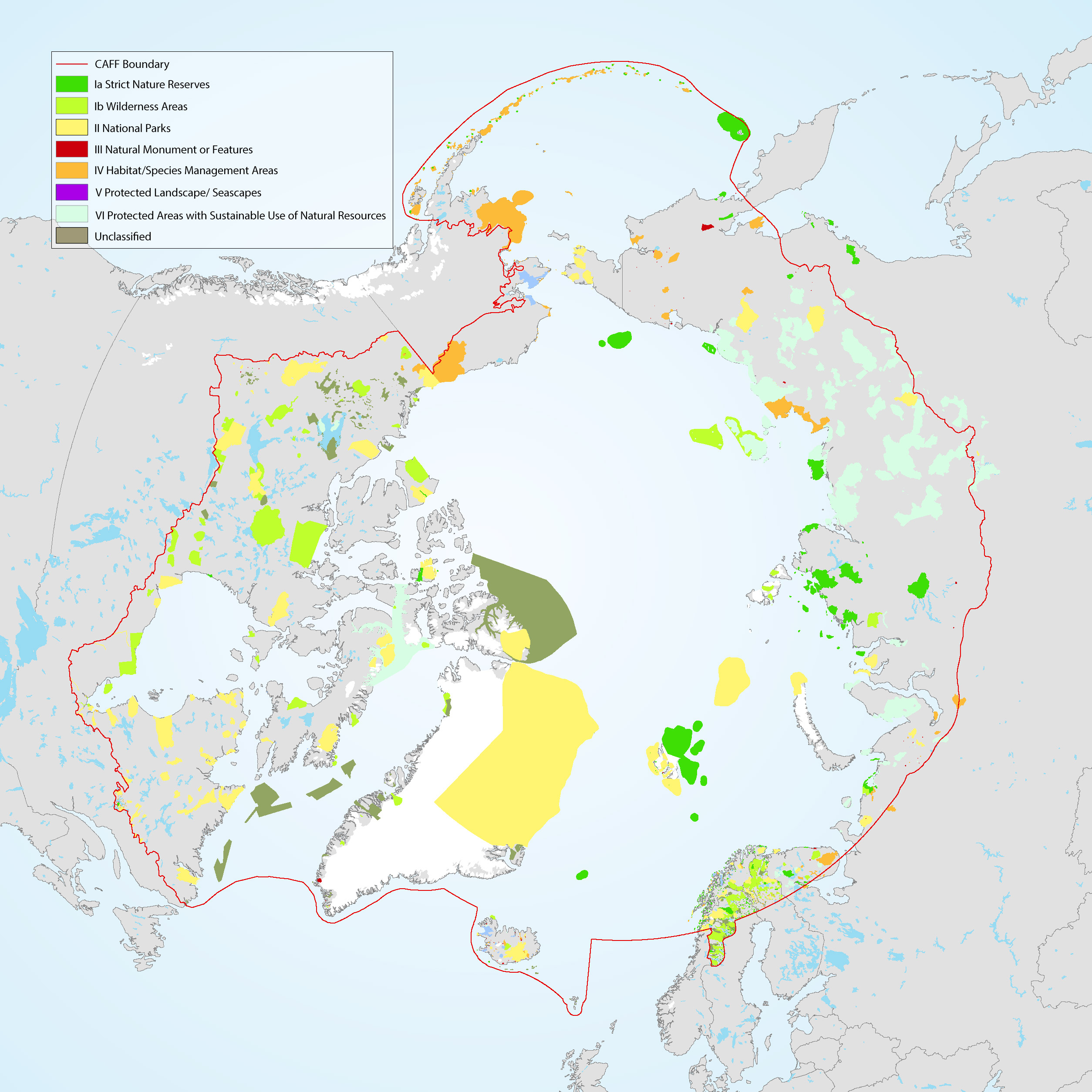
The Conservation of Arctic Flora and Fauna (CAFF) and Protection of the Arctic Marine Environment (PAME) working groups of the Arctic Council developed this update on the 2017 indicator report (CAFF-PAME 2017). It provides an overview of the status and trends of protected areas in the Arctic and an overview of Other Effective area-based Conservation Measures. The data used represents the results of the 2020 update to the Arctic Protected Areas Database submitted by each of the Arctic Council member states.
-
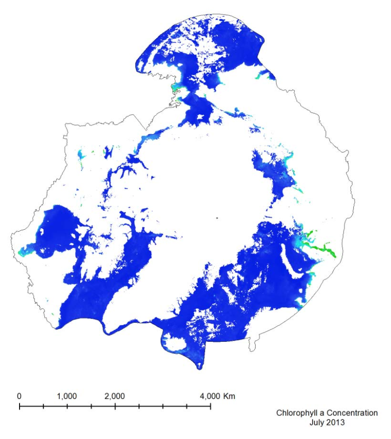
The MODIS marine chlorophyll a product provided, similar to SST, is a 4 km global monthly composite based on smaller resolution daily imagery compiled by NASA. The imagery is reliant on clear ocean (free of clouds and ice) so only months from March to October have been provided, as the chlorophyll levels in the Arctic diminish during the winter months, when sea ice is prevalent. The marine chlorophyll a is measured in mg/m3
-
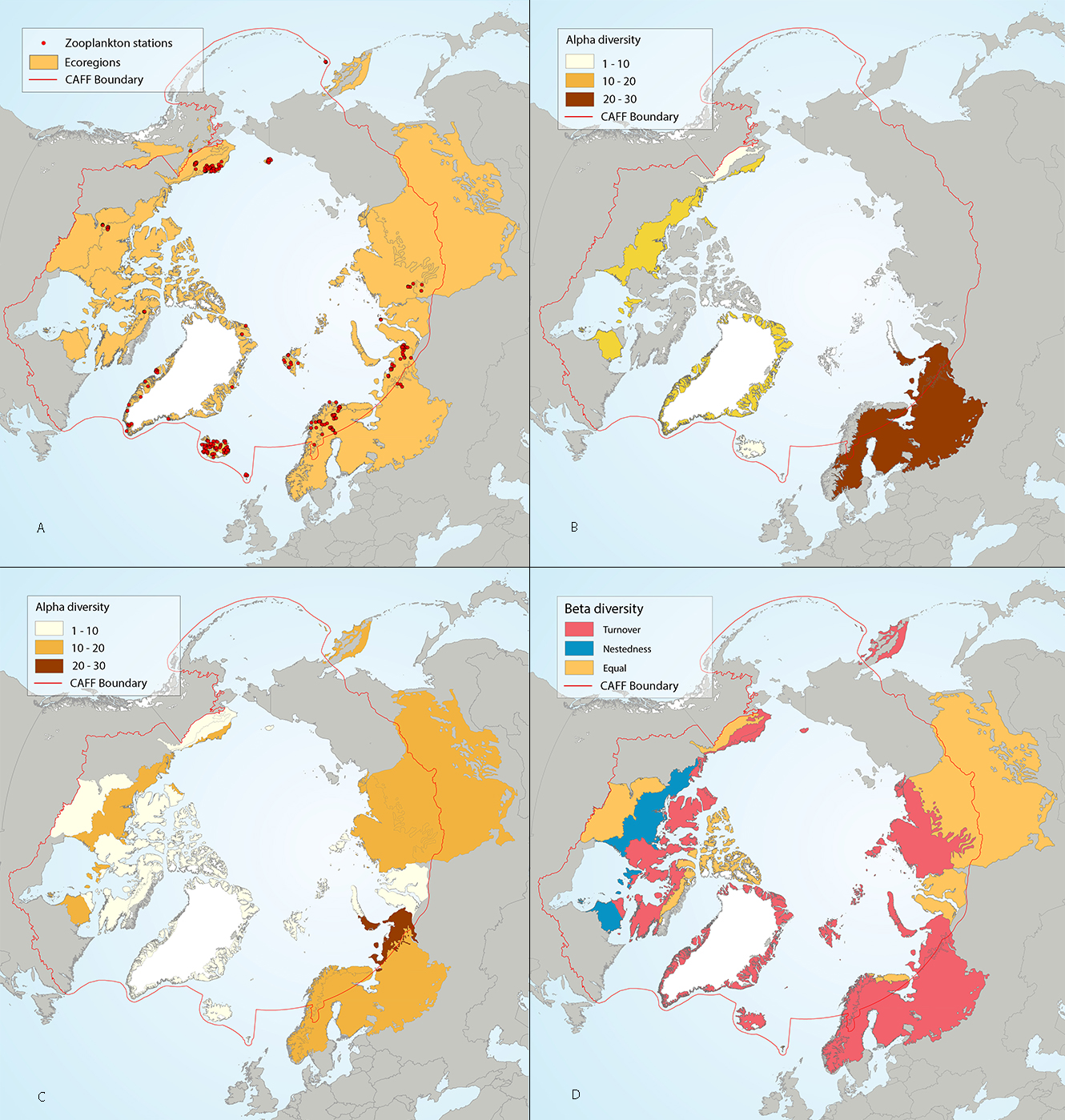
Results of circumpolar assessment of lake zooplankton, focused just on crustaceans, and indicating (a) the location of crustacean zooplankton stations, underlain by circumpolar ecoregions; (b) ecoregions with many crustacean zooplankton stations, colored on the basis of alpha diversity rarefied to 25 stations; (c) all ecoregions with crustacean zooplankton stations, colored on the basis of alpha diversity rarefied to 10 stations; (d) ecoregions with at least two stations in a hydrobasin, colored on the basis of the dominant component of beta diversity (species turnover, nestedness, approximately equal contribution, or no diversity) when averaged across hydrobasins in each ecoregion. State of the Arctic Freshwater Biodiversity Report - Chapter 4 - Page 58 - Figure 4-25
-
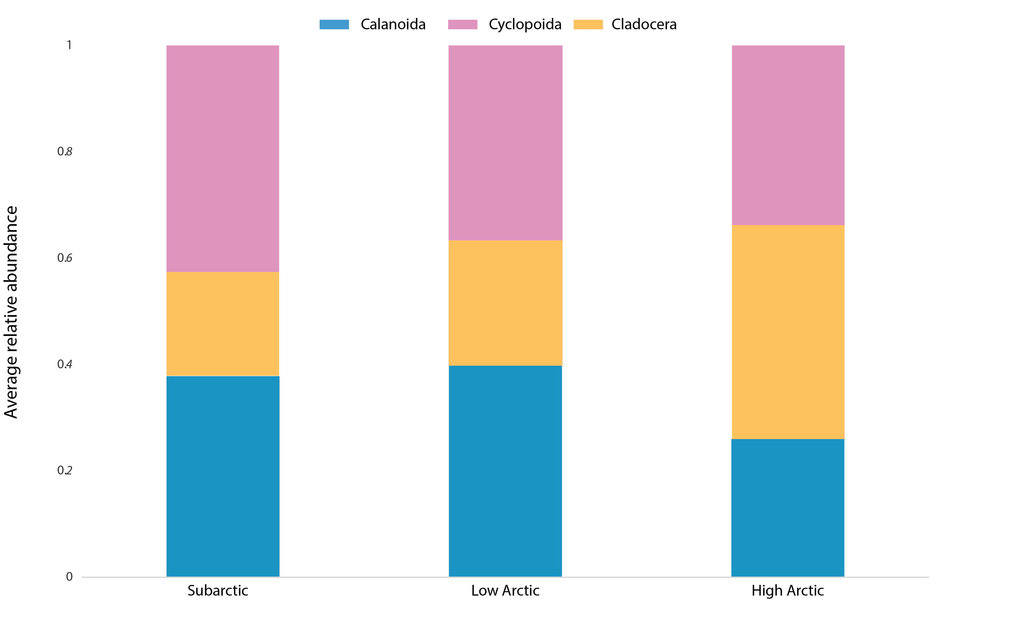
Average relative abundance of the main zooplankton groups (calanoid copepods, cyclopoid copepods, cladocerans) for the sub-Arctic (n=150), low- Arctic (n=154), and high-Arctic (n=55) regions. Samples with a single taxon have been excluded. State of the Arctic Freshwater Biodiversity Report - Chapter 4 - Page 61 - Figure 4-28