 CAFF - Arctic Biodiversity Data Service (ABDS)
Type of resources
Available actions
Topics
Keywords
Contact for the resource
Provided by
Years
Formats
Representation types
Update frequencies
status
Service types
Scale
-
The Seabird Information Network (SIN) developed by the Circumpolar Seabird expert group (<a href="http://caff.is/seabirds-cbird" target="_blank">CBird</a>) of the Conservation of Arctic Flora and Fauna (<a href="http://caff.is" target="_blank">CAFF</a>) working group of the Arctic Council focuses on the development of a data entry and analysis portal system allowing for circumpolar seabird colony information to be contributed, mapped, and shared by scientists and monitoring programs around the Arctic. - <a href="http://axiom.seabirds.net/maps/js/seabirds.php?app=circumpolar#z=2&ll=NaN,0.00000" target="_blank"> Circumpolar Seabird portal</a>
-
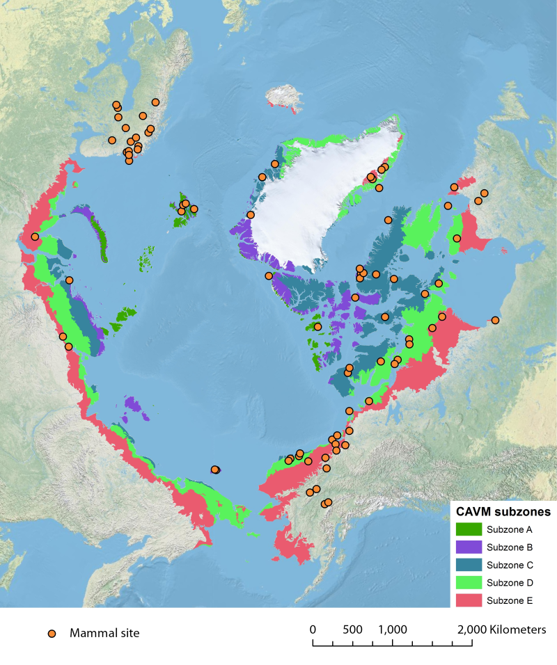
Location of long-term mammal monitoring sites and programs. Comes from the Arctic Terrestrial Biodiversity Monitoring Plan is developed to improve the collective ability of Arctic traditional knowledge holders, northern communities and scientists to detect, understand and report on long-term change in Arctic terrestrial ecosystems and biodiversity..
-
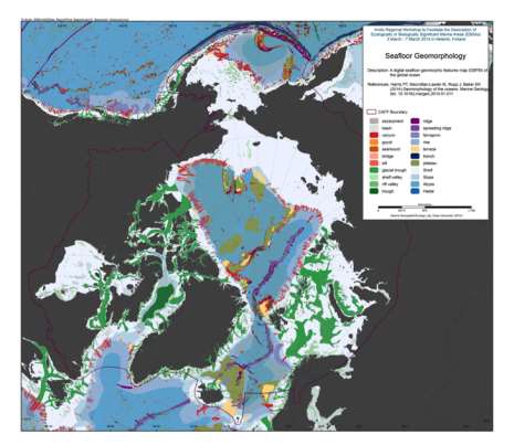
We present the first digital seafloor geomorphic features map (GSFM) of the global ocean. The GSFM includes 131,192 separate polygons in 29 geomorphic feature categories, used here to assess differences between passive and active continental margins as well as between 8 major ocean regions (the Arctic, Indian, North Atlantic, North Pacific, South Atlantic, South Pacific and the Southern Oceans and the Mediterranean and Black Seas). The GSFM provides quantitative assessments of differences between passive and active margins: continental shelf width of passive margins (88 km) is nearly three times that of active margins (31 km); the average width of active slopes (36 km) is less than the average width of passive margin slopes (46 km); active margin slopes contain an area of 3.4 million km2 where the gradient exceeds 5°, compared with 1.3 million km2 on passive margin slopes; the continental rise covers 27 million km2 adjacent to passive margins and less than 2.3 million km2 adjacent to active margins. Examples of specific applications of the GSFM are presented to show that: 1) larger rift valley segments are generally associated with slow-spreading rates and smaller rift valley segments are associated with fast spreading; 2) polar submarine canyons are twice the average size of non-polar canyons and abyssal polar regions exhibit lower seafloor roughness than non-polar regions, expressed as spatially extensive fan, rise and abyssal plain sediment deposits – all of which are attributed here to the effects of continental glaciations; and 3) recognition of seamounts as a separate category of feature from ridges results in a lower estimate of seamount number compared with estimates of previous workers. Reference: Harris PT, Macmillan-Lawler M, Rupp J, Baker EK Geomorphology of the oceans. Marine Geology.
-
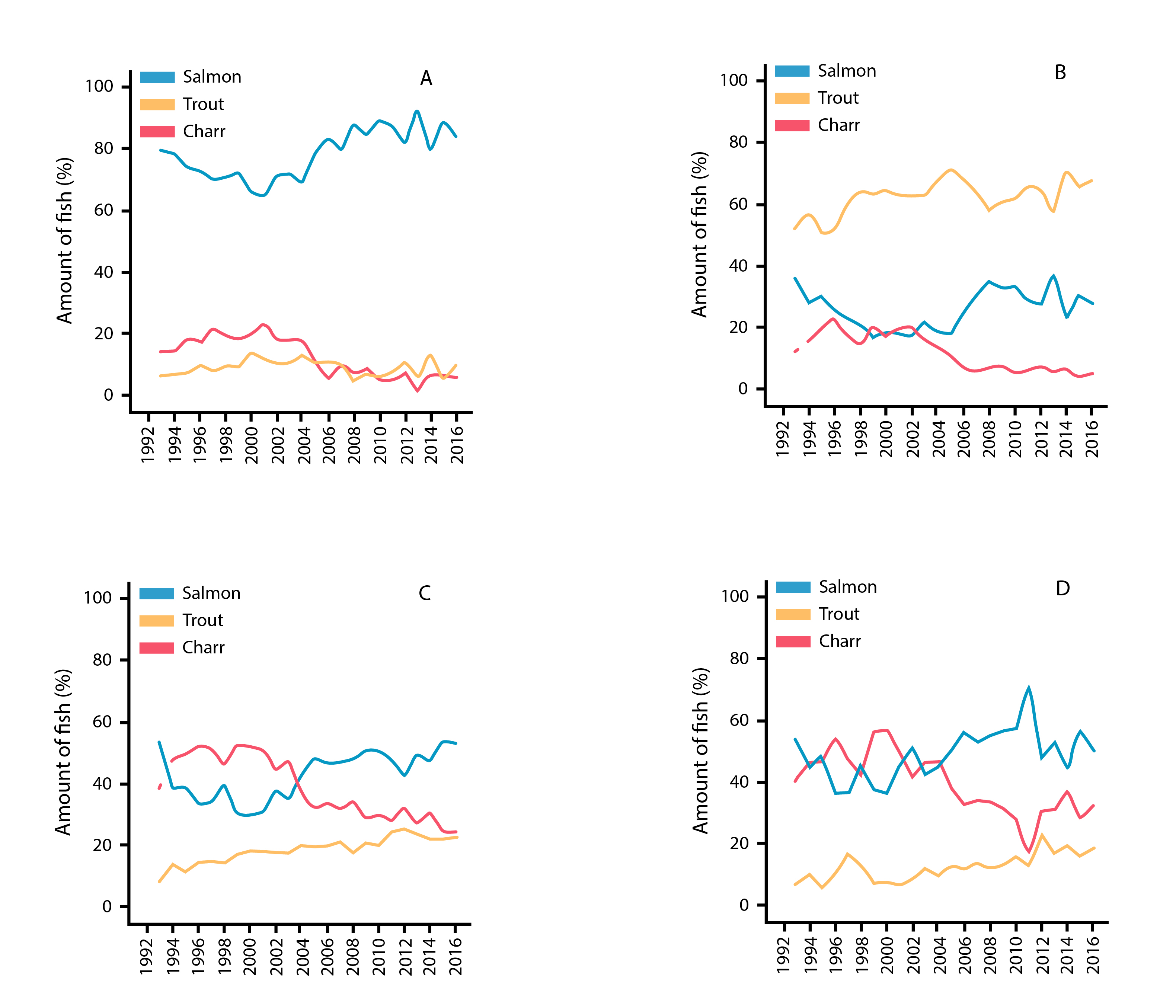
Temporal patterns in % abundance of Atlantic salmon, brown trout, and anadromous Arctic charr from catch statistics in Iceland rivers monitored from 1992 to 2016, showing results from (a) west, (b) south, (c) north, and (d) east Iceland. State of the Arctic Freshwater Biodiversity Report - Chapter 4 - Page 81 - Figure 4-41
-
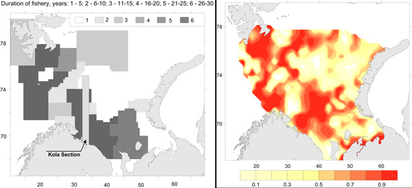
Commercial fishery impact on zoobenthos of the Barents Sea. Figure A) Intensity and duration of fishery efforts in standard commercial fishery areas in the Barents Sea. The darker the area the longer the fishery has been in operation. Figure B) Level of decline in macrobenthic biomass between 1926-1932 and 1968-1970 calculated as 1-b1968/b1930. The largest biomass decreases correspond to the darker colour, whereas lighter colour refers to no change (Denisenko 2013). STATE OF THE ARCTIC MARINE BIODIVERSITY REPORT - <a href="https://arcticbiodiversity.is/findings/benthos" target="_blank">Chapter 3</a> - Page 97 - Figure 3.3.4
-
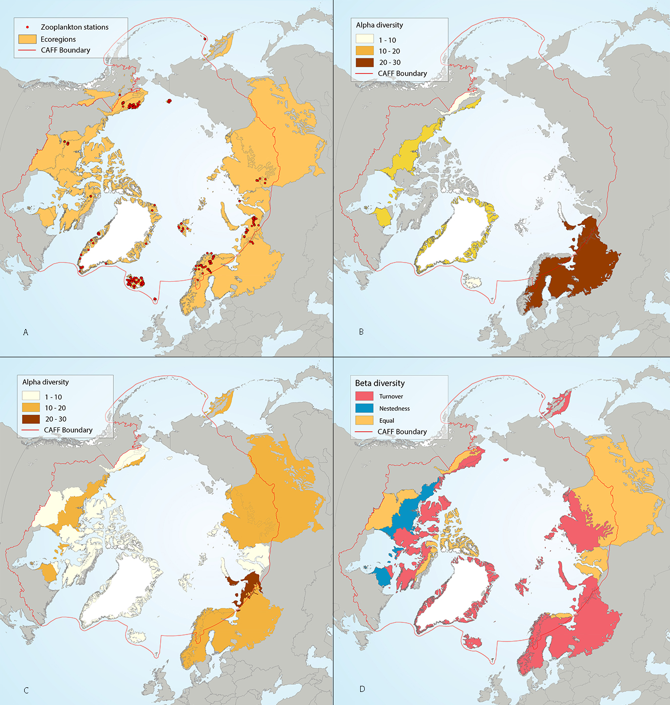
Results of circumpolar assessment of lake zooplankton, focused just on crustaceans, and indicating (a) the location of crustacean zooplankton stations, underlain by circumpolar ecoregions; (b) ecoregions with many crustacean zooplankton stations, colored on the basis of alpha diversity rarefied to 25 stations; (c) all ecoregions with crustacean zooplankton stations, colored on the basis of alpha diversity rarefied to 10 stations; (d) ecoregions with at least two stations in a hydrobasin, colored on the basis of the dominant component of beta diversity (species turnover, nestedness, approximately equal contribution, or no diversity) when averaged across hydrobasins in each ecoregion. State of the Arctic Freshwater Biodiversity Report - Chapter 4 - Page 58 - Figure 4-25
-
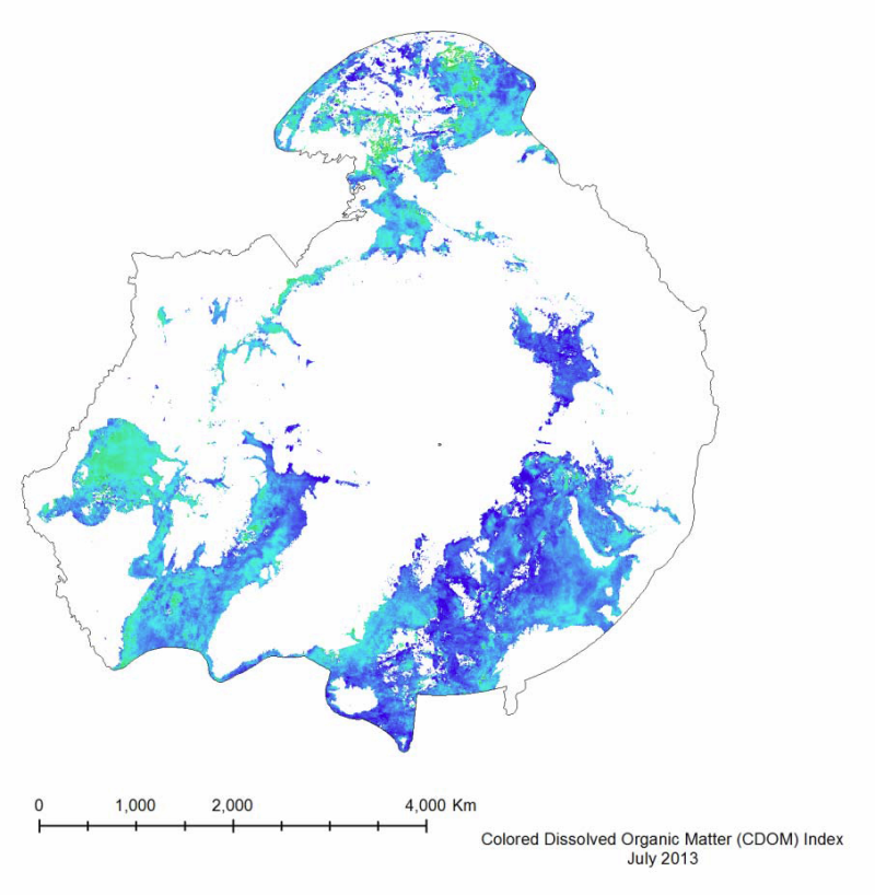
Colored Dissolved Organic Matter (CDOM) is a measurement of the absorption of light in the UV and visible spectrum by the colored components of dissolved organic carbon. It is essentially the yellow substance in water as a result of decaying detritus. It is important to measure because it limits the amount of sunlight penetration, and thus restricts the growth of plankton populations. It is measured in a unit-less CDOM index. Data generated as part of CAFFs Circumpolar Biodiversity Monitoring Program (CAFF) and its Land Cover Change Initiative (LCC) Trends visible in the MODIS dataset show an overall decrease in the mean CDOM from 2003 to 2012, with a percent change of -31.7%. This trend can be seen in Figure 40. This decrease corresponds to the increase in total yearly primary productivity (Figure 30), as a decrease in the CDOM allows for sunlight to penetrate deeper into the water, boosting chlorophyll concentrations and thus primary productivity.
-
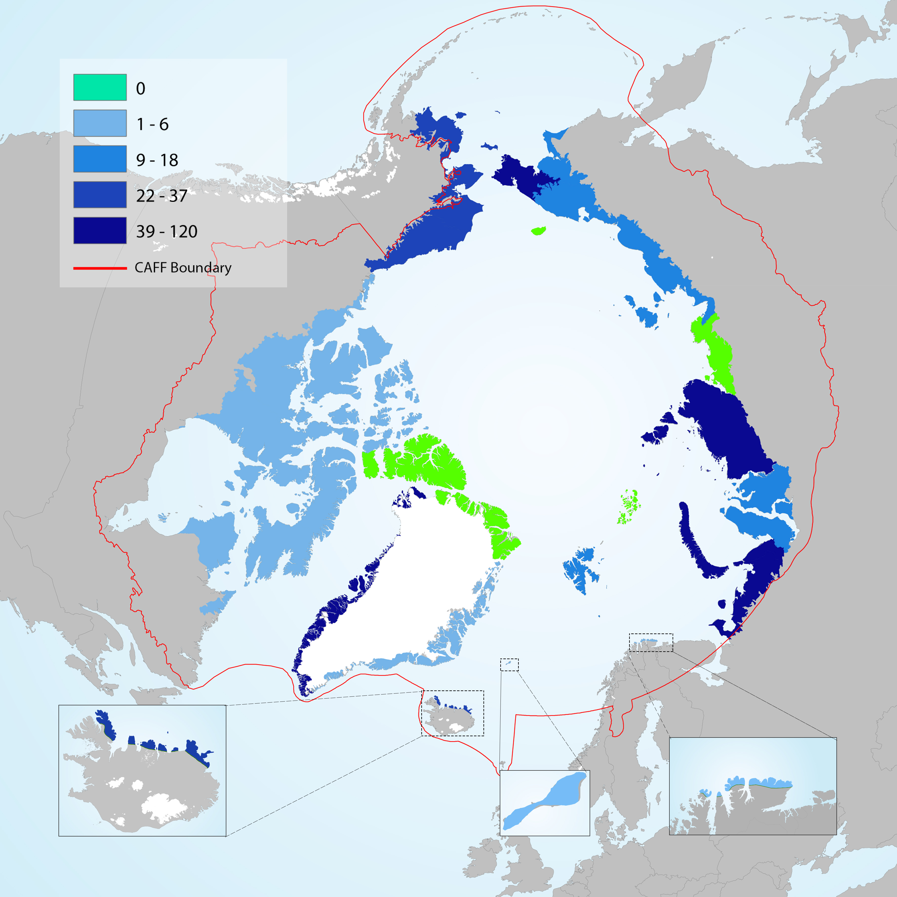
Number of non-native plant taxa that have become naturalised across the Arctic. No naturalised non-native taxa are recorded from Wrangel Island, Ellesmere Land – northern Greenland, Anabar-Olenyok and Frans Josef Land. Modified from Wasowicz et al. 2020 STATE OF THE ARCTIC TERRESTRIAL BIODIVERSITY REPORT - Chapter 3 - Page 32 - Figure 3.4
-
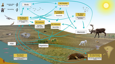
Conceptual model of the FECs and processes mediated by more than 2,500 species of Arctic arthropods known from Greenland, Iceland, Svalbard, and Jan Mayen. STATE OF THE ARCTIC TERRESTRIAL BIODIVERSITY REPORT - Chapter 3 - Page 37- Figure 3.7
-
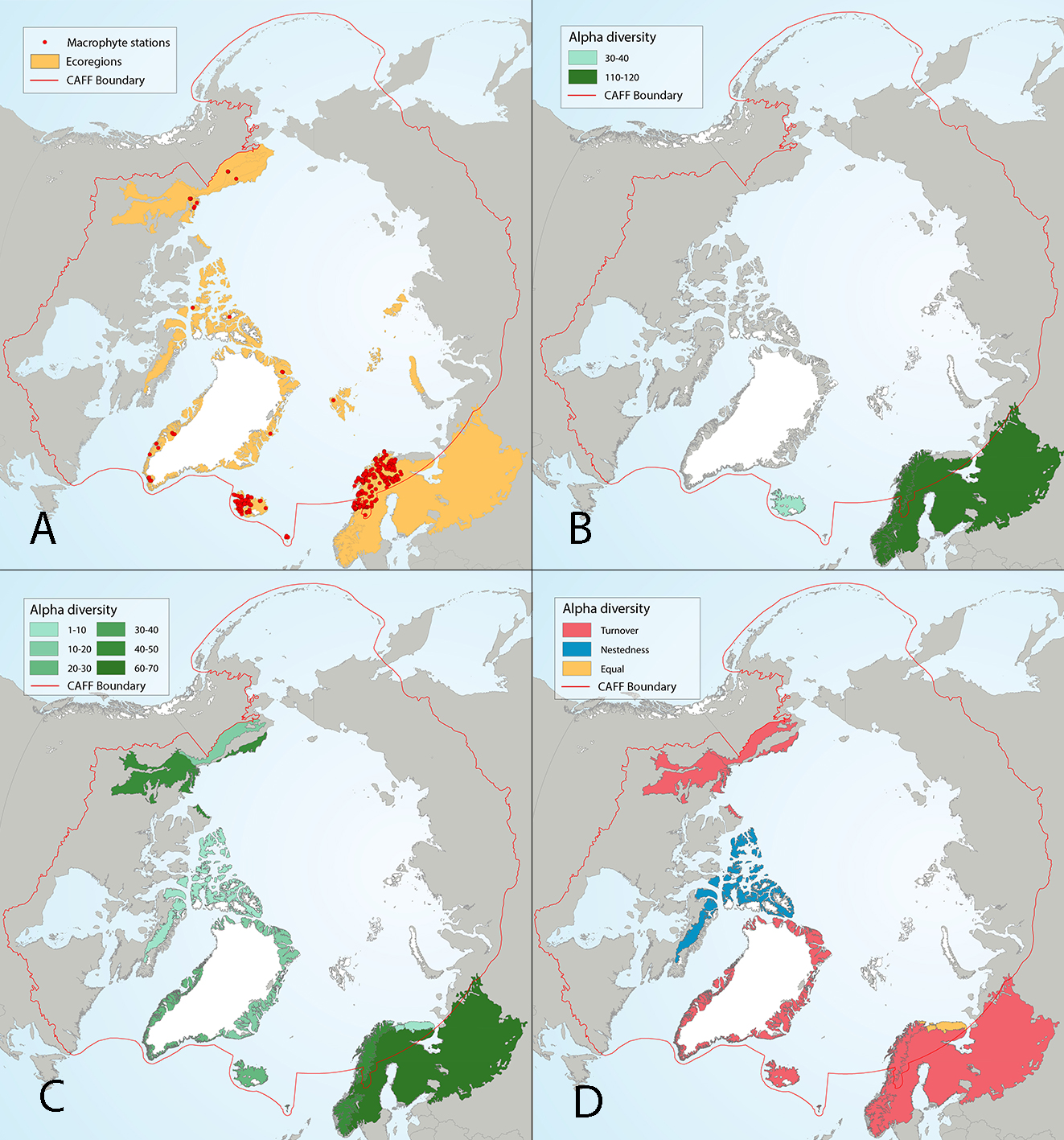
Figure 4 22 Results of circumpolar assessment of lake macrophytes, indicating (a) the location of macrophyte stations, underlain by circumpolar ecoregions; (b) ecoregions with many macrophyte stations, colored on the basis of alpha diversity rarefied to 70 stations; (c) all ecoregions with macrophyte stations, colored on the basis of alpha diversity rarefied to 10 stations; (d) ecoregions with at least two stations in a hydrobasin, colored on the basis of the dominant component of beta diversity (species turnover, nestedness, approximately equal contribution, or no diversity) when averaged across hydrobasins in each ecoregion. State of the Arctic Freshwater Biodiversity Report - Chapter 4 - Page 54 - Figure 4-22