 CAFF - Arctic Biodiversity Data Service (ABDS)
Type of resources
Available actions
Topics
Keywords
Contact for the resource
Provided by
Years
Formats
Representation types
Update frequencies
status
Service types
Scale
-
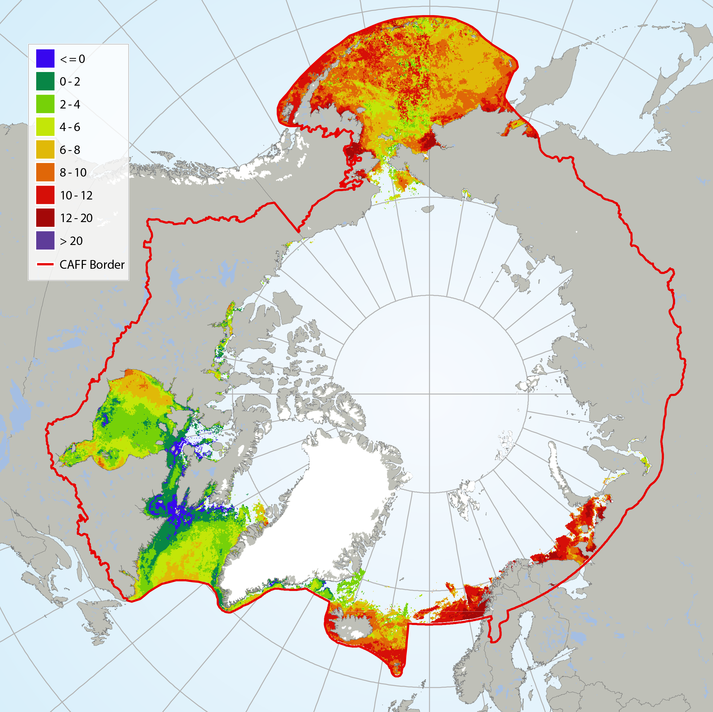
It has not been possible to identify available trend data for Arctic Ocean sea surface temperatures because there is not enough data to calculate reliable long-term trends for much of the Arctic marine environment (IPCC 2013, NOAA 2015). Here, sea surface temperature for July 2015 is shown from CAFF’s Land Cover Change Index. MODIS Sea Surface Temperature (SST) provided a four-kilometre spatial resolution monthly composite snapshot made from night-time measurements from the NASA Aqua Satellite. The night-time measurements are used to collect a consistent temperature measurement that is unaffected by the warming of the top layer of water by the sun. STATE OF THE ARCTIC MARINE BIODIVERSITY REPORT - <a href="https://arcticbiodiversity.is/marine" target="_blank">Chapter 2</a> - Page 25 - Figure 2.3
-
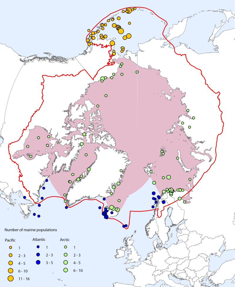
<img src="http://geo.abds.is/geonetwork/srv/eng//resources.get?uuid=59d822e4-56ce-453c-b98d-40207a2e9eec&fname=cbmp_small.png" alt="logo" height="67px" align="left" hspace="10px"> The Arctic marine data set contains a total of 111 species and 310 population time series from 170 locations. Species coverage is about 34% of Arctic marine vertebrate species (100% of mammals, 53% of birds, and 27% of fishes) (Bluhm et al. 2011). At the species level, even though the representation of Arctic fish species is lower than that of mammals and birds, the data are dominated by fishes, primarily from the Pacific Ocean (especially the Bering Sea and Aleutian Islands). However, there are more population time series in total for bird species, which is reflective of this group being both better studied historically and also monitored at many small study sites compared to fish and marine mammal species, which are regularly monitored at a much larger scale through stock management. Note that the time span selected for marine analyses is 1970 to 2005 (compared with 1970 to 2007 for the ASTI for all species). CAFF Assessment Series No. 7 April 2012 - <a href=http://caff.is/asti/asti-publications/28-arctic-species-trend-index-tracking-trends-in-arctic-marine-populations" target="_blank"> The Arctic Species Trend Index - Tracking trends in Arctic marine populations </a>
-
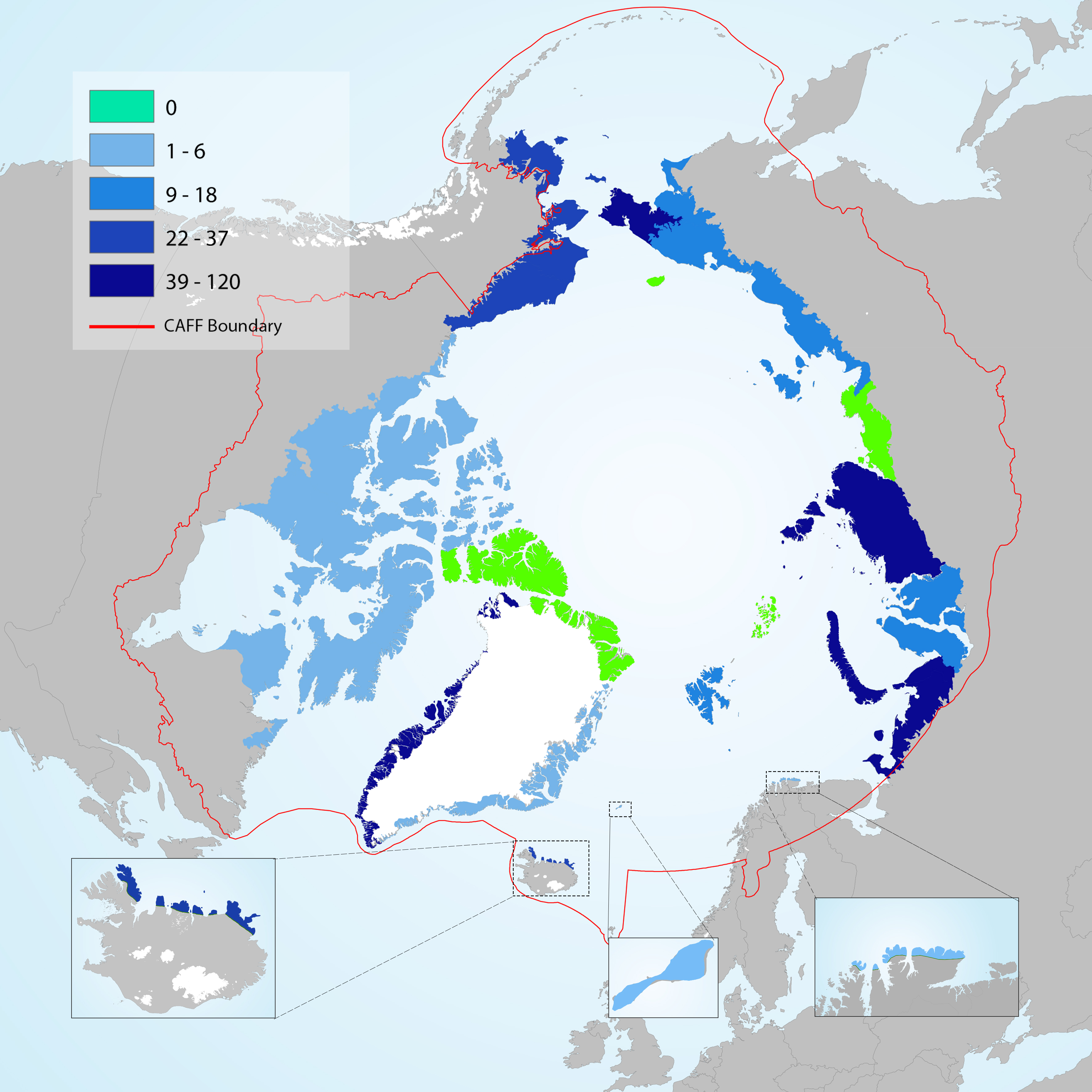
Number of non-native plant taxa that have become naturalised across the Arctic. No naturalised non-native taxa are recorded from Wrangel Island, Ellesmere Land – northern Greenland, Anabar-Olenyok and Frans Josef Land. Modified from Wasowicz et al. 2020 STATE OF THE ARCTIC TERRESTRIAL BIODIVERSITY REPORT - Chapter 3 - Page 32 - Figure 3.4
-
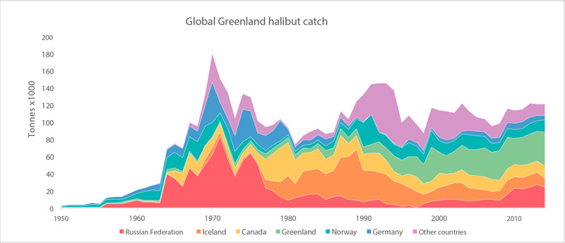
Global catches of Greenland halibut (FAO 2015). STATE OF THE ARCTIC MARINE BIODIVERSITY REPORT - <a href="https://arcticbiodiversity.is/findings/marine-fishes" target="_blank">Chapter 3</a> - Page 121 - Figure 3.4.8
-

Interannual differences in taxonomic composition of phytoplankton during summer in a) Kongsfjorden and b) Rijpfjorden (Source: MOSJ, Norwegian Polar Institute). STATE OF THE ARCTIC MARINE BIODIVERSITY REPORT - <a href="https://arcticbiodiversity.is/findings/plankton" target="_blank">Chapter 3</a> - Page 74 - Figure 3.2.5
-
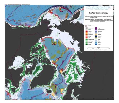
We present the first digital seafloor geomorphic features map (GSFM) of the global ocean. The GSFM includes 131,192 separate polygons in 29 geomorphic feature categories, used here to assess differences between passive and active continental margins as well as between 8 major ocean regions (the Arctic, Indian, North Atlantic, North Pacific, South Atlantic, South Pacific and the Southern Oceans and the Mediterranean and Black Seas). The GSFM provides quantitative assessments of differences between passive and active margins: continental shelf width of passive margins (88 km) is nearly three times that of active margins (31 km); the average width of active slopes (36 km) is less than the average width of passive margin slopes (46 km); active margin slopes contain an area of 3.4 million km2 where the gradient exceeds 5°, compared with 1.3 million km2 on passive margin slopes; the continental rise covers 27 million km2 adjacent to passive margins and less than 2.3 million km2 adjacent to active margins. Examples of specific applications of the GSFM are presented to show that: 1) larger rift valley segments are generally associated with slow-spreading rates and smaller rift valley segments are associated with fast spreading; 2) polar submarine canyons are twice the average size of non-polar canyons and abyssal polar regions exhibit lower seafloor roughness than non-polar regions, expressed as spatially extensive fan, rise and abyssal plain sediment deposits – all of which are attributed here to the effects of continental glaciations; and 3) recognition of seamounts as a separate category of feature from ridges results in a lower estimate of seamount number compared with estimates of previous workers. Reference: Harris PT, Macmillan-Lawler M, Rupp J, Baker EK Geomorphology of the oceans. Marine Geology.
-
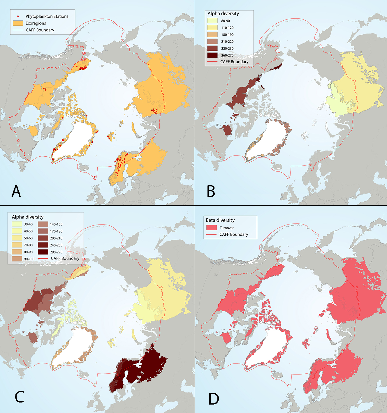
Figure 4 17 Results of circumpolar assessment of lake phytoplankton,(a) the location of phytoplankton stations, underlain by circumpolar ecoregions; (b) ecoregions with many phytoplankton stations, colored on the basis of alpha diversity rarefied to 35 stations; (c) all ecoregions with phytoplankton stations, colored on the basis of alpha diversity rarefied to 10 stations; (d) ecoregions with at least two stations in a hydrobasin, colored on the basis of the dominant component of beta diversity (species turnover, nestedness, approximately equal contribution, or no diversity) when averaged across hydrobasins in each ecoregion. State of the Arctic Freshwater Biodiversity Report - Chapter 4 - Page 56 - Figure 4-17
-
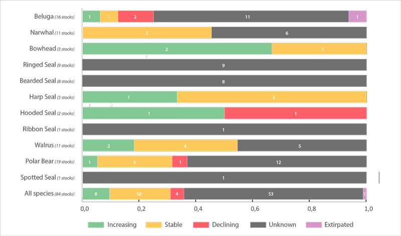
Trends in abundance of Arctic marine mammal Focal Ecosystem Components based on the most recent assessment for each recognized subpopulation of a species (red, declining trend; yellow, stable trend; green, increasing trend; grey, unknown trend). Number of subpopulations is given after species name. Each column is divided into equal segments, the sizes of which are not proportional to the size of the subpopulation. Ringed seal and bearded seal segments represent subspecies. Walrus segments represent subpopulations within subspecies. See Table 3.6.1 for details on abundance. STATE OF THE ARCTIC MARINE BIODIVERSITY REPORT - <a href="https://arcticbiodiversity.is/findings/marine-mammals" target="_blank">Chapter 3</a> - Page 156 - Figure 3.6.2
-
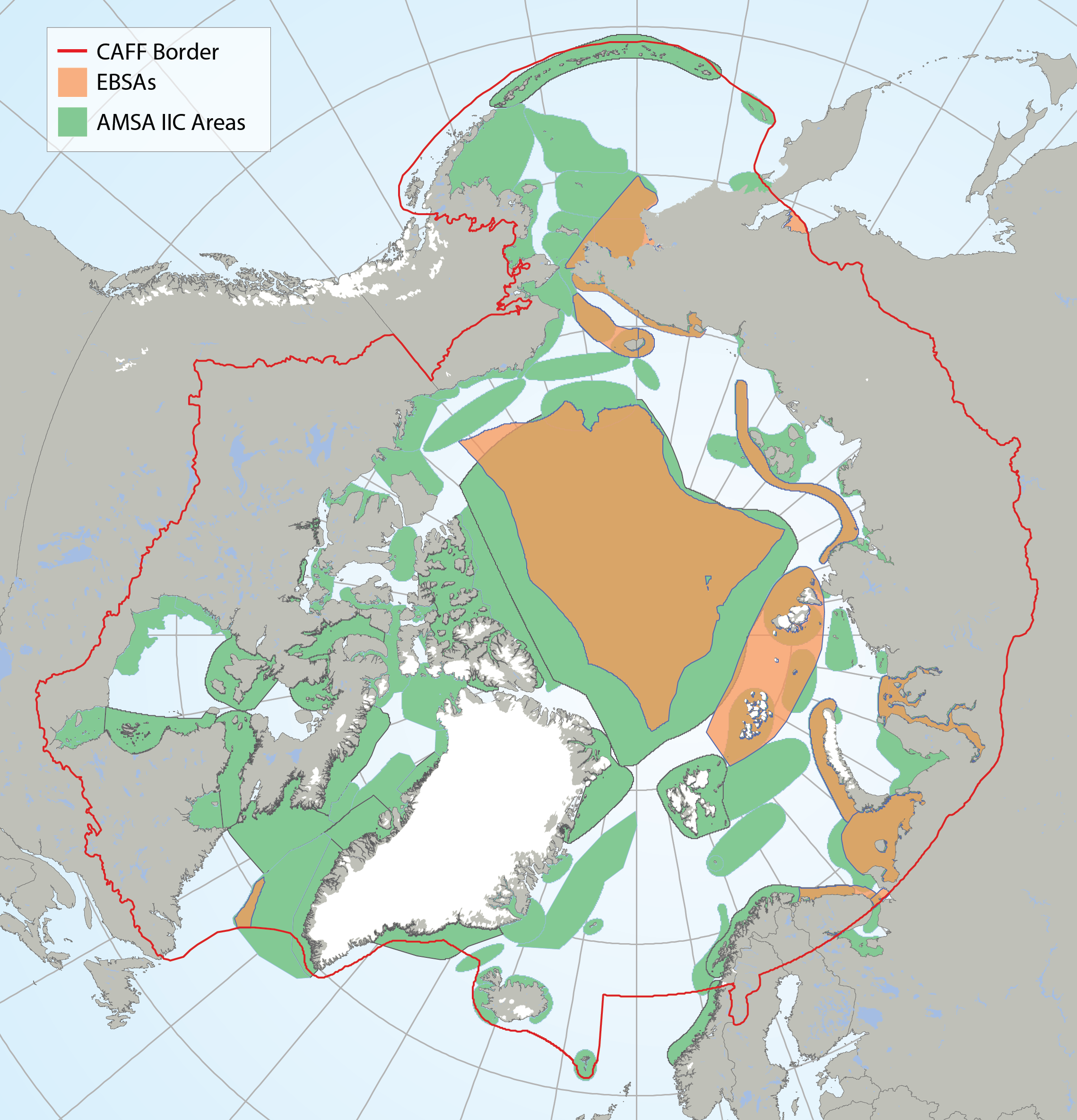
Arctic Ecologically and Biologically Significant Areas (EBSAs) and Arctic Marine Areas of Heightened Ecological and Cultural Significance as identified in the Arctic Marine Shipping Assessment (AMSA) IIC report. STATE OF THE ARCTIC MARINE BIODIVERSITY REPORT - <a href="https://arcticbiodiversity.is/marine" target="_blank">Chapter 1</a> - Page 16 - Box Figure 1.1
-
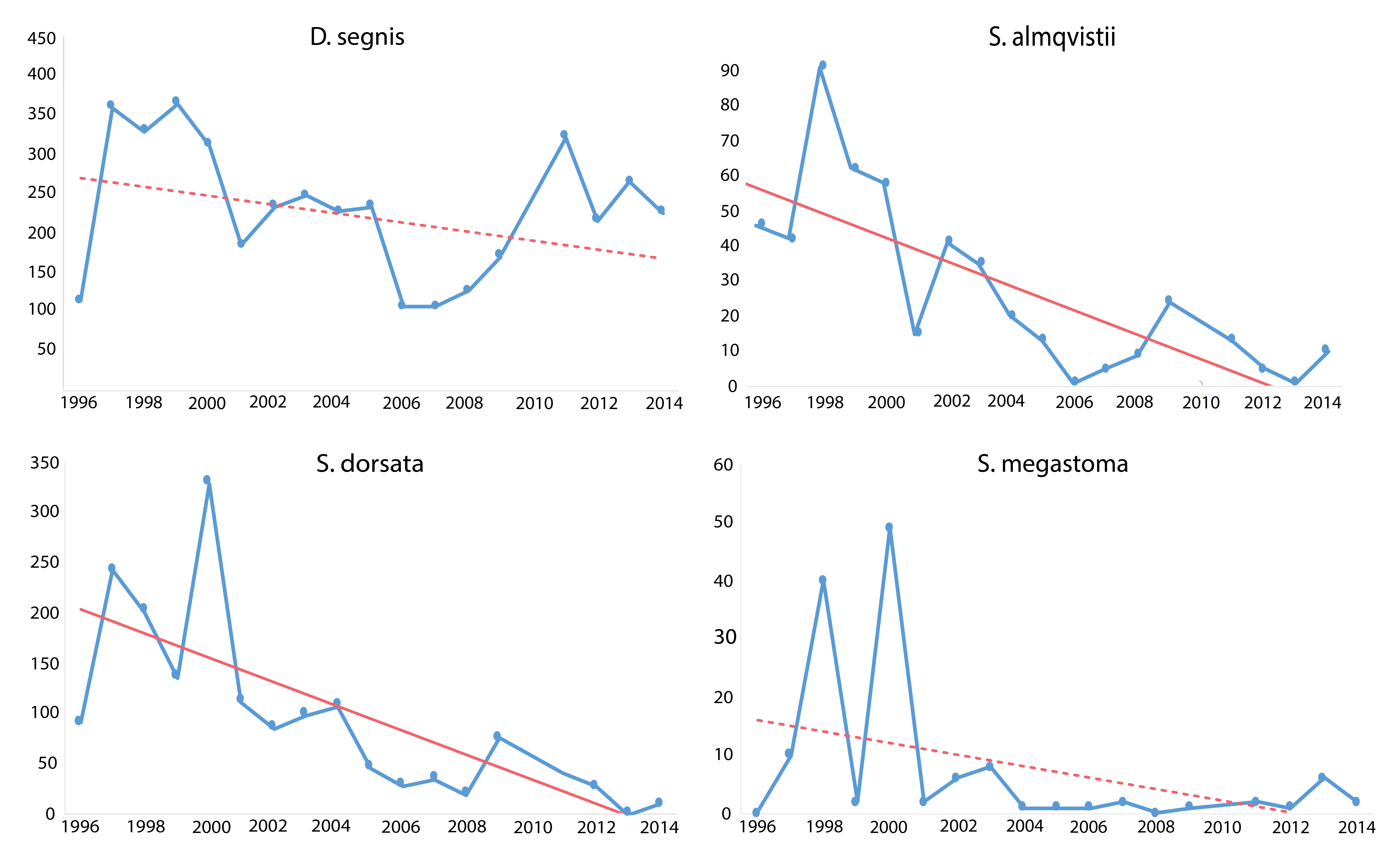
Trends in four muscid species occurring at Zackenberg Research Station, east Greenland, 1996–2014. Declines were detected in several species over five or more years. Significant regression lines drawn as solid. Non-significant as dotted lines. Modified from Gillespie et al. 2020a. (in the original figure six species showed a statistically significant decline, seven a non-significant decline and one species a non-significant rise) STATE OF THE ARCTIC TERRESTRIAL BIODIVERSITY REPORT - Chapter 3 - Page 39 - Figure 3.11