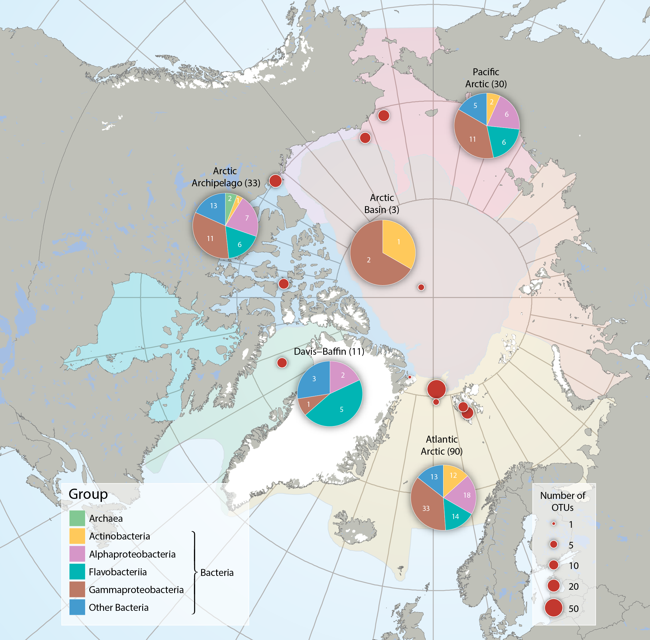
Bacteria and Archaea across five Arctic Marine Areas based on number of operational taxonomic units (OTUs), or molecular species. Composition of microbial groups, with respective numbers of OTUs (pie charts) and number of OTUs at sampling locations (red dots). Data aggregated by the CBMP Sea Ice Biota Expert Network. Data source: National Center for Biotechnology Information’s (NCBI 2017) Nucleotide and PubMed databases. STATE OF THE ARCTIC MARINE BIODIVERSITY REPORT - <a href="https://arcticbiodiversity.is/findings/sea-ice-biota" target="_blank">Chapter 3</a> - Page 38 - Figure 3.1.2 From the report draft: "Synthesis of available data was performed by using searches conducted in the National Center for Biotechnology Information’s “Nucleotide” (http://www.ncbi.nlm.nih.gov/guide/data-software/) and “PubMed” (http://www.ncbi.nlm.nih.gov/pubmed) databases. Aligned DNA sequences were downloaded and clustered into OTUs by maximum likelihood phylogenetic placement."

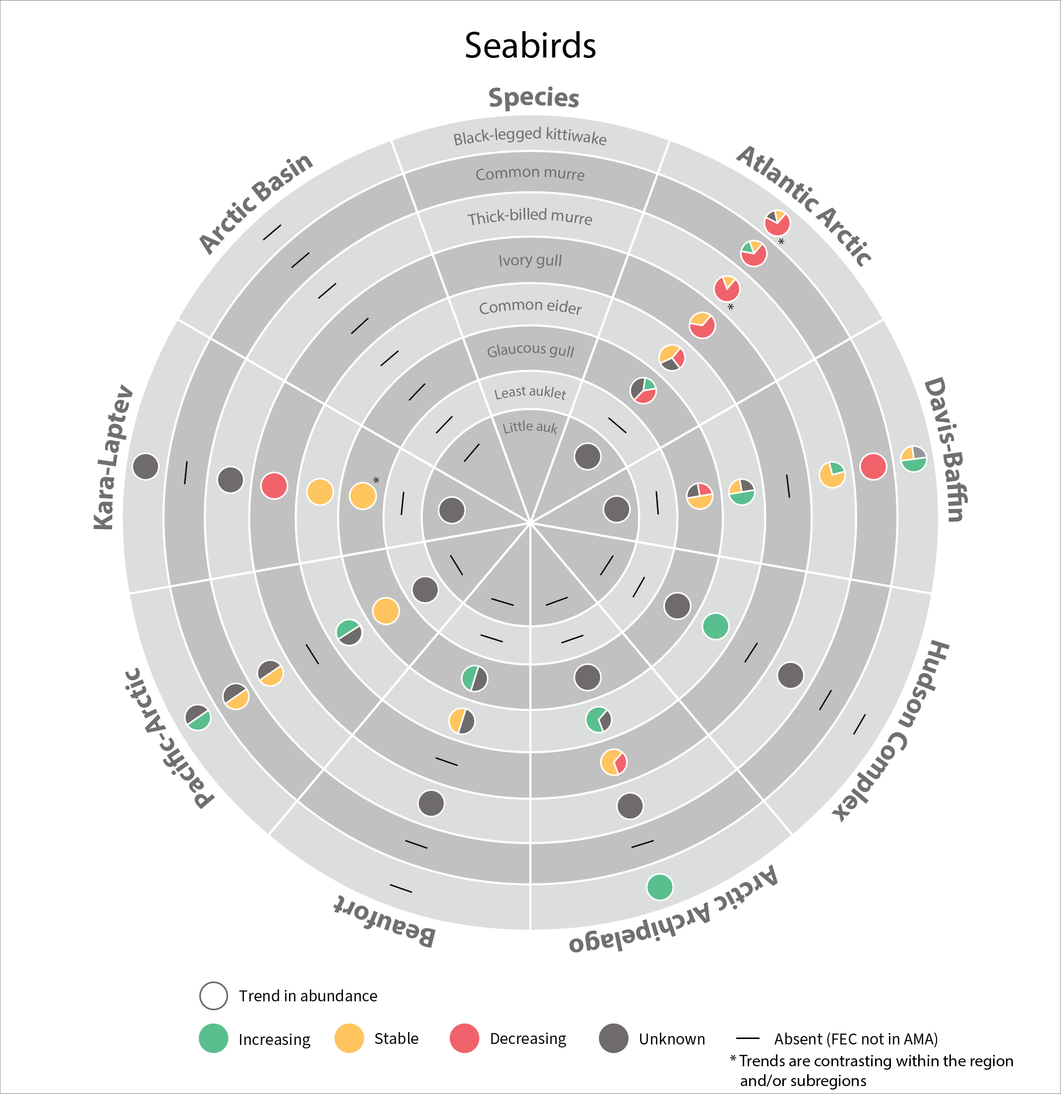
In 2017, the SAMBR synthesized data about biodiversity in Arctic marine ecosystems around the circumpolar Arctic. SAMBR highlighted observed changes and relevant monitoring gaps using data compiled through 2015. In 2021 an update was provided on the status of seabirds in circumpolar Arctic using data from 2016–2019. Most changes reflect access to improved population estimates, orimproved data for monitoring trends,independent of recognized trends in population size.

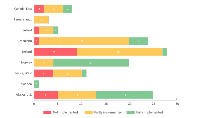
The number of key sites (monitored colonies) for seabirds (in 22 CSMP ecoregions) by country (a total of 125 sites). Sites are categorized as having fully, partially, or not met the CSMP criteria for parameters monitored (see 2.6.2). Data were from Appendix 3 of the CSMP (Irons et al. 2015); the degree of implementation may have changed at some sites since this summary was compiled. STATE OF THE ARCTIC MARINE BIODIVERSITY REPORT - <a href="https://arcticbiodiversity.is/findings/seabirds" target="_blank">Chapter 3</a> - Page 134 - Figure 3.5.2

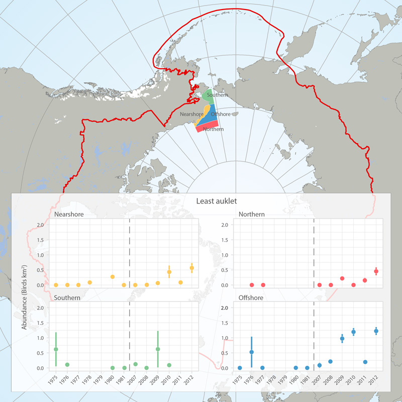
Abundance (birds/km2) of least auklets in four regions (see map) of the eastern Chukchi Sea, 1975-1981 and 2007-2012, based on at-sea surveys (archived in the North Pacific Pelagic Seabird Database). Figures provided by Adrian Gall, ABR, Inc. and reprinted with permission. STATE OF THE ARCTIC MARINE BIODIVERSITY REPORT - <a href="https://arcticbiodiversity.is/findings/seabirds" target="_blank">Chapter 3</a> - Page 138 - Box fig. 3.5.1 The shapefile outlines 4 regions of the eastern Chukchi Sea that were surveyed for seabirds during the open-water seasons of 1976-2012. We compared the density of seabirds in these regions among two time periods (1975-1981 and 2008-2012) to assess changes in seabird abundance over the past 4 decades. We also include a figure showing abundance of Least Auklets 1975-2012. Data are from the North Pacific Pelagic Seabird Database, maintained by the USGS (http://alaska.usgs.gov/science/biology/nppsd/index.php).

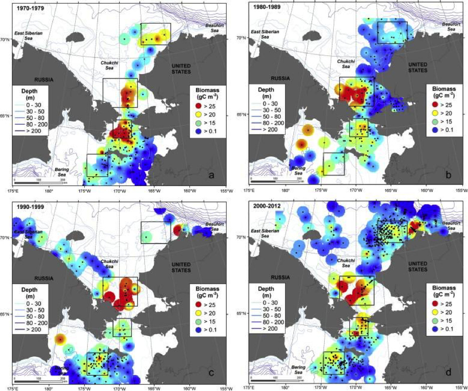
Benthic macro-infauna biomass in the northern Bering and Chukchi Seas from 1970 to 2012, displayed as decadal pattern Adapted from Grebmeier et al. (2015a) with permission from Elsevier. STATE OF THE ARCTIC MARINE BIODIVERSITY REPORT - <a href="https://arcticbiodiversity.is/findings/benthos" target="_blank">Chapter 3</a> - Page 98 - Figure 3.3.6 Cumulative scores of benthos drivers for each of the 8 CAFF-AMAs. The cumulative scores are taken from the last column of Table 3.3.1. The flower chart/plot helps to visualize the data.

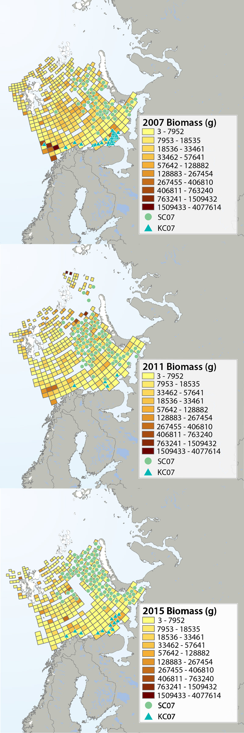
Megafauna distribution of biomass (g/15 min trawling) in the Barents Sea in 2007, 2011 and 2015. The green circles show the distribution of the snow crab as it spreads from east to west, and the blue triangles show the invasion of king crab along the coast of the southern Barents Sea. Data from Institute of Marine Research, Norway and the Polar Research Institute of Marine Fisheries and Oceanography, Murmansk, Russia. STATE OF THE ARCTIC MARINE BIODIVERSITY REPORT - <a href="https://arcticbiodiversity.is/findings/benthos" target="_blank">Chapter 3</a> - Page 95 - Figure 3.3.2 The annual joint Norwegian–Russian Ecosystem Survey provides from more than 400 stations and during extensive cruise tracks covering more or less the whole Barents Sea in August– September. The sampling is based on a regular grid spanning about 1.5 millionkm2 with fixed positions of stations which make it possible to measure changes in spatial distribution over time. The trawl is a Campelen 1800 bottom trawl rigged with rock-hopper groundgear and towed on double Warps. The mesh size is 80 mm (stretched) in the front and 16–22 mmin the cod end, allowing the capture and retention of smaller fish and the largest benthos from the seabed (benthic megafauna). The horizontal opening was 11.7 m, and the vertical opening 4–5 m (Teigsmark and Øynes, 1982). The trawl configuration and bottom contact was monitored remotely by SCANMAR trawl sensors. The standard distance between trawl stations was 35 nautical miles (65 km), except north and west of Svalbard where a stratified sampling was adapted to the steep continental shelve. The standard procedure was to tow 15 min after the trawl had made contact with the bottom, but the actual tow duration ranged between 5 min and 1 h and data were subsequently standardized to 15 min trawl time. Towing speed was 3 knots, equivalent to a towing distance of 0.75 nautical miles (1.4 km) during a 15 min tow. The trawl catches were recorded using the same procedures on the Russian and the Norwegian Research vessels to ensure comparability across Barents Sea regions. The benthic megafauna was separated from the fish and shrimp catch, washed, and sorted to lowest possible taxonomic level, in most cases to species, on-Board the vessel. Species identification was standardized between the researcher teams by annually exchanging the benthic expert’s among the vessels and taxon names were fixed each year according toWORMSwhen possible.This resulted in an Electronic identification manual and photo-compendium as a tool to standardize taxon identifications, in addition to various sources of identification literature. Difficult taxa were photographed and, in some cases, brought back as preserved voucher specimens for further identification. Wet-weight biomass was recorded with electronic scales in the ship laboratories for each taxon.The biomass determination included all fragments.

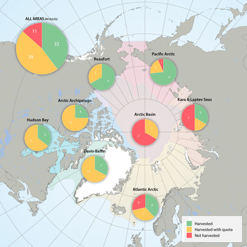
Harvest marine mammal Focal Ecosystem Component stocks in Arctic Marine Areas. Harvested without quotas, with quotas or not harvested. STATE OF THE ARCTIC MARINE BIODIVERSITY REPORT - <a href="https://arcticbiodiversity.is/findings/marine-mammals" target="_blank">Chapter 3</a> - Page 158 - Figure 3.6.4

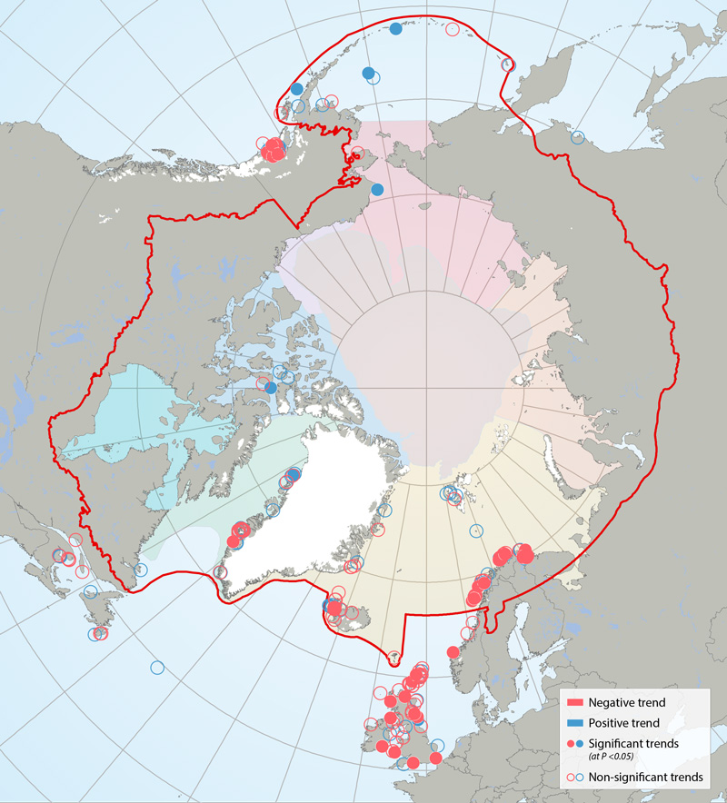
Trends in kittiwake colonies 2001-2010, based on linear regression with year as the explanatory variable. Slope of the regression is red = negative trend, blue = positive trend; shaded circle = significant trend (at p<0.05), open circle = non-significant trend. Non-significant deviation from zero could imply a stable population, but in some cases was due to low sample size and low power. Provided with permission from Descamps et al. (in prep). STATE OF THE ARCTIC MARINE BIODIVERSITY REPORT - <a href="https://arcticbiodiversity.is/findings/seabirds" target="_blank">Chapter 3</a> - Page 135 - Figure 3.5.3 This figure is compiled from data from researchers working throughout circumpolar regions, primarily members of the Circumpolar Seabird Group, an EN of CAFF/seabirds. Dr. Sebastien Decamps conducted the analysis and produced the original figure; the full results will be available in an article in prep titled: “Descamps et al. in prep. Circumpolar dynamics of black-legged kittiwakes track large-scale environmental shifts and oceans' warming rate.” [expected submission spring 2016]. Colony population trends were analyzed using a linear regression with the year as explanatory variable. Based on slope of the regression (which cannot be exactly 0) colonies are either Declining (Slope of the regression <0) or Increasing (Slope of the regression >0). (Colonies may have had a negative but not significant slope, and could be stable but for some others, the slope is not significant due to small sample size / low power; thus we cannot say that all colonies with a non- significant slope are stable. The threshold was put at 5% to assess the significance of the trend.

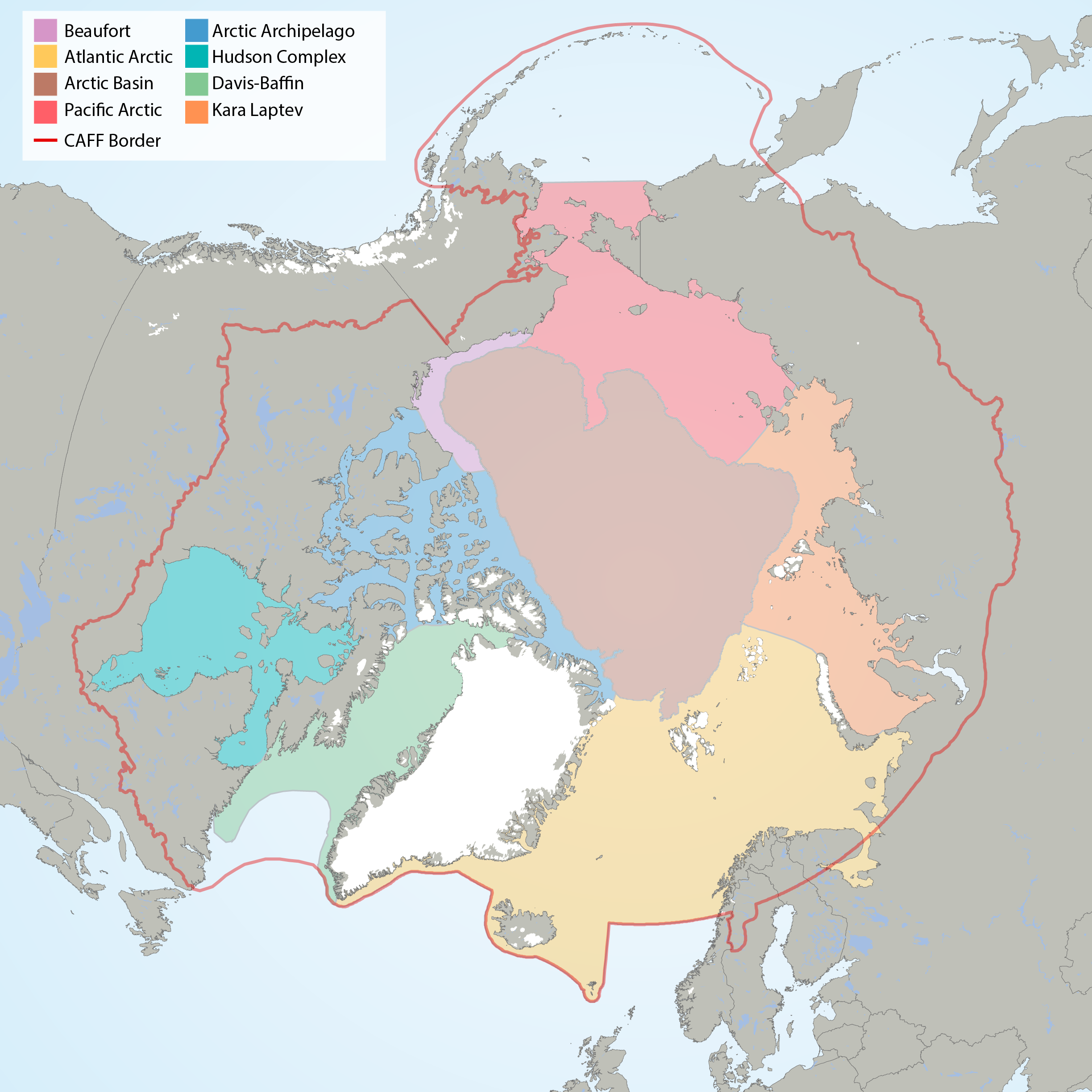
Arctic Marine Areas (AMAs) as defined in the CBMP Marine Plan. STATE OF THE ARCTIC MARINE BIODIVERSITY REPORT - <a href="https://arcticbiodiversity.is/marine" target="_blank">Chapter 1</a> - Page 15 - Figure 1.2

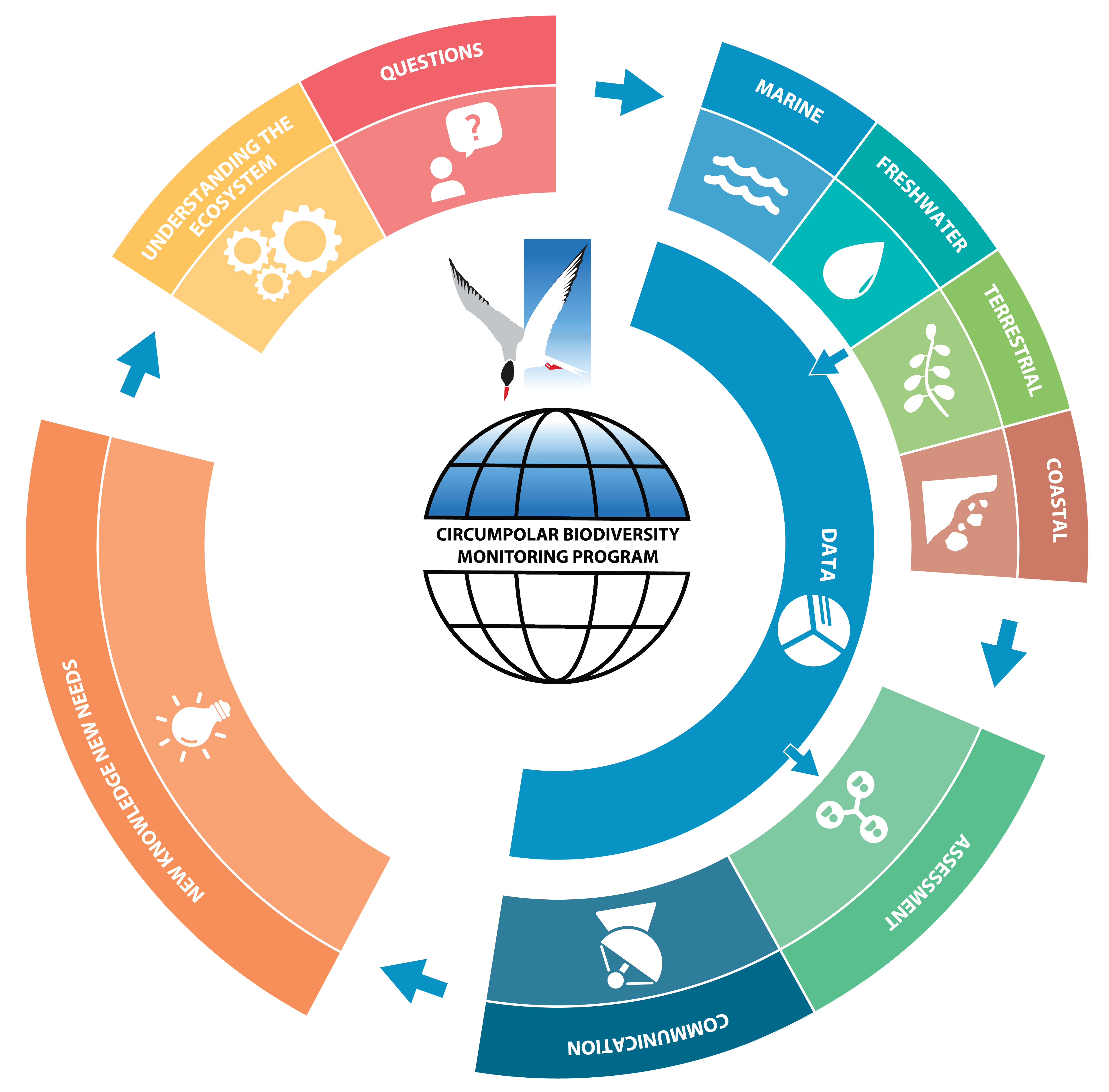
Workflow of the Circumpolar Biodiversity Monitoring Program (CBMP). STATE OF THE ARCTIC MARINE BIODIVERSITY REPORT - <a href="https://arcticbiodiversity.is/marine" target="_blank">Chapter 1</a> - Page 13 - Figure 1.1