 CAFF - Arctic Biodiversity Data Service (ABDS)
asNeeded
Type of resources
Available actions
Topics
Keywords
Contact for the resource
Provided by
Years
Formats
Representation types
Update frequencies
status
Scale
-
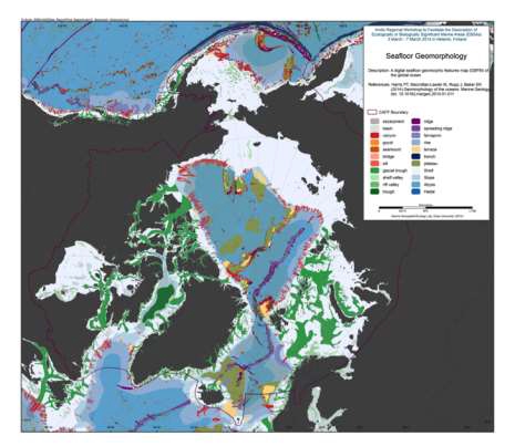
We present the first digital seafloor geomorphic features map (GSFM) of the global ocean. The GSFM includes 131,192 separate polygons in 29 geomorphic feature categories, used here to assess differences between passive and active continental margins as well as between 8 major ocean regions (the Arctic, Indian, North Atlantic, North Pacific, South Atlantic, South Pacific and the Southern Oceans and the Mediterranean and Black Seas). The GSFM provides quantitative assessments of differences between passive and active margins: continental shelf width of passive margins (88 km) is nearly three times that of active margins (31 km); the average width of active slopes (36 km) is less than the average width of passive margin slopes (46 km); active margin slopes contain an area of 3.4 million km2 where the gradient exceeds 5°, compared with 1.3 million km2 on passive margin slopes; the continental rise covers 27 million km2 adjacent to passive margins and less than 2.3 million km2 adjacent to active margins. Examples of specific applications of the GSFM are presented to show that: 1) larger rift valley segments are generally associated with slow-spreading rates and smaller rift valley segments are associated with fast spreading; 2) polar submarine canyons are twice the average size of non-polar canyons and abyssal polar regions exhibit lower seafloor roughness than non-polar regions, expressed as spatially extensive fan, rise and abyssal plain sediment deposits – all of which are attributed here to the effects of continental glaciations; and 3) recognition of seamounts as a separate category of feature from ridges results in a lower estimate of seamount number compared with estimates of previous workers. Reference: Harris PT, Macmillan-Lawler M, Rupp J, Baker EK Geomorphology of the oceans. Marine Geology.
-

Locations and associated attributes of circumpolar Muskox studies. Attributes include animal count, population estimate, estimate error and associated report citation.
-

We present the first digital seafloor geomorphic features map (GSFM) of the global ocean. The GSFM includes 131,192 separate polygons in 29 geomorphic feature categories, used here to assess differences between passive and active continental margins as well as between 8 major ocean regions (the Arctic, Indian, North Atlantic, North Pacific, South Atlantic, South Pacific and the Southern Oceans and the Mediterranean and Black Seas). The GSFM provides quantitative assessments of differences between passive and active margins: continental shelf width of passive margins (88 km) is nearly three times that of active margins (31 km); the average width of active slopes (36 km) is less than the average width of passive margin slopes (46 km); active margin slopes contain an area of 3.4 million km2 where the gradient exceeds 5°, compared with 1.3 million km2 on passive margin slopes; the continental rise covers 27 million km2 adjacent to passive margins and less than 2.3 million km2 adjacent to active margins. Examples of specific applications of the GSFM are presented to show that: 1) larger rift valley segments are generally associated with slow-spreading rates and smaller rift valley segments are associated with fast spreading; 2) polar submarine canyons are twice the average size of non-polar canyons and abyssal polar regions exhibit lower seafloor roughness than non-polar regions, expressed as spatially extensive fan, rise and abyssal plain sediment deposits – all of which are attributed here to the effects of continental glaciations; and 3) recognition of seamounts as a separate category of feature from ridges results in a lower estimate of seamount number compared with estimates of previous workers. Reference: Harris PT, Macmillan-Lawler M, Rupp J, Baker EK Geomorphology of the oceans. Marine Geology.
-
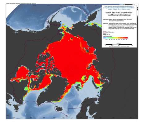
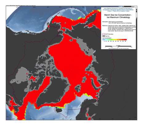
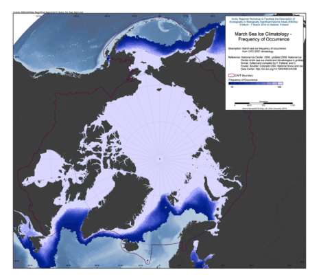
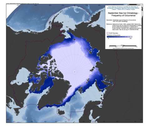
The U.S. National Ice Center (NIC) is an inter-agency sea ice analysis and forecasting center comprised of the Department of Commerce/NOAA, the Department of Defense/U.S. Navy, and the Department of Homeland Security/U.S. Coast Guard components. Since 1972, NIC has produced Arctic and Antarctic sea ice charts. This data set is comprised of Arctic sea ice concentration climatology derived from the NIC weekly or biweekly operational ice-chart time series. The charts used in the climatology are from 1972 through 2007; and the monthly climatology products are median, maximum, minimum, first quartile, and third quartile concentrations, as well as frequency of occurrence of ice at any concentration for the entire period of record as well as for 10-year and 5-year periods. NIC charts are produced through the analyses of available in situ, remote sensing, and model data sources. They are generated primarily for mission planning and safety of navigation. NIC charts generally show more ice than do passive microwave derived sea ice concentrations, particularly in the summer when passive microwave algorithms tend to underestimate ice concentration. The record of sea ice concentration from the NIC series is believed to be more accurate than that from passive microwave sensors, especially from the mid-1990s on (see references at the end of this documentation), but it lacks the consistency of some passive microwave time series. Source: <a href="http://nsidc.org/data/G02172" target="_blank">NSIDC</a> Reference: National Ice Center. 2006, updated 2009. National Ice Center Arctic sea ice charts and climatologies in gridded format. Edited and compiled by F. Fetterer and C. Fowler. Boulder, Colorado USA: National Snow and Ice Data Center. Source: <a href="http://nsidc.org/data/G02172" target="_blank">NSIDC</a>
-
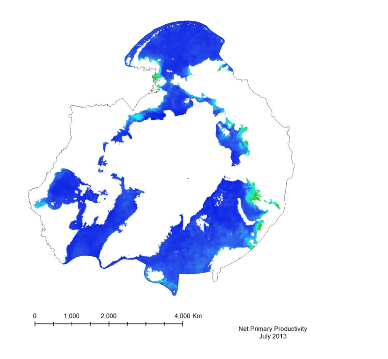
Marine primary productivity is not available from the NASA Ocean Color website. Currently the best product available for marine primary productivity is available through Oregon State University’s Ocean Productivity Project. A monthly global Net Primary Productivity product at 9 km spatial resolution has been selected for this analysis. The algorithm used to create the primary productivity is a Vertically Generalized Production Model (VGPM) created by Behrenfeld and Falkowski (1997). It is a “chlorophyll-based” model that estimates net primary production from chlorophyll using a temperature-dependent description of chlorophyll photosynthetic efficiency (O’Malley 2010). Inputs to the function are chlorophyll, available light, and photosynthetic efficiency.
-
The U.S. National Ice Center (NIC) is an inter-agency sea ice analysis and forecasting center comprised of the Department of Commerce/NOAA, the Department of Defense/U.S. Navy, and the Department of Homeland Security/U.S. Coast Guard components. Since 1972, NIC has produced Arctic and Antarctic sea ice charts. This data set is comprised of Arctic sea ice concentration climatology derived from the NIC weekly or biweekly operational ice-chart time series. The charts used in the climatology are from 1972 through 2007; and the monthly climatology products are median, maximum, minimum, first quartile, and third quartile concentrations, as well as frequency of occurrence of ice at any concentration for the entire period of record as well as for 10-year and 5-year periods. NIC charts are produced through the analyses of available in situ, remote sensing, and model data sources. They are generated primarily for mission planning and safety of navigation. NIC charts generally show more ice than do passive microwave derived sea ice concentrations, particularly in the summer when passive microwave algorithms tend to underestimate ice concentration. The record of sea ice concentration from the NIC series is believed to be more accurate than that from passive microwave sensors, especially from the mid-1990s on (see references at the end of this documentation), but it lacks the consistency of some passive microwave time series. Source: <a href="http://nsidc.org/data/G02172" target="_blank">NSIDC</a> Reference: National Ice Center. 2006, updated 2009. National Ice Center Arctic sea ice charts and climatologies in gridded format. Edited and compiled by F. Fetterer and C. Fowler. Boulder, Colorado USA: National Snow and Ice Data Center. Source: <a href="http://nsidc.org/data/G02172" target="_blank">NSIDC</a>
-

We present the first digital seafloor geomorphic features map (GSFM) of the global ocean. The GSFM includes 131,192 separate polygons in 29 geomorphic feature categories, used here to assess differences between passive and active continental margins as well as between 8 major ocean regions (the Arctic, Indian, North Atlantic, North Pacific, South Atlantic, South Pacific and the Southern Oceans and the Mediterranean and Black Seas). The GSFM provides quantitative assessments of differences between passive and active margins: continental shelf width of passive margins (88 km) is nearly three times that of active margins (31 km); the average width of active slopes (36 km) is less than the average width of passive margin slopes (46 km); active margin slopes contain an area of 3.4 million km2 where the gradient exceeds 5°, compared with 1.3 million km2 on passive margin slopes; the continental rise covers 27 million km2 adjacent to passive margins and less than 2.3 million km2 adjacent to active margins. Examples of specific applications of the GSFM are presented to show that: 1) larger rift valley segments are generally associated with slow-spreading rates and smaller rift valley segments are associated with fast spreading; 2) polar submarine canyons are twice the average size of non-polar canyons and abyssal polar regions exhibit lower seafloor roughness than non-polar regions, expressed as spatially extensive fan, rise and abyssal plain sediment deposits – all of which are attributed here to the effects of continental glaciations; and 3) recognition of seamounts as a separate category of feature from ridges results in a lower estimate of seamount number compared with estimates of previous workers. Reference: Harris PT, Macmillan-Lawler M, Rupp J, Baker EK Geomorphology of the oceans. Marine Geology.
-
The U.S. National Ice Center (NIC) is an inter-agency sea ice analysis and forecasting center comprised of the Department of Commerce/NOAA, the Department of Defense/U.S. Navy, and the Department of Homeland Security/U.S. Coast Guard components. Since 1972, NIC has produced Arctic and Antarctic sea ice charts. This data set is comprised of Arctic sea ice concentration climatology derived from the NIC weekly or biweekly operational ice-chart time series. The charts used in the climatology are from 1972 through 2007; and the monthly climatology products are median, maximum, minimum, first quartile, and third quartile concentrations, as well as frequency of occurrence of ice at any concentration for the entire period of record as well as for 10-year and 5-year periods. NIC charts are produced through the analyses of available in situ, remote sensing, and model data sources. They are generated primarily for mission planning and safety of navigation. NIC charts generally show more ice than do passive microwave derived sea ice concentrations, particularly in the summer when passive microwave algorithms tend to underestimate ice concentration. The record of sea ice concentration from the NIC series is believed to be more accurate than that from passive microwave sensors, especially from the mid-1990s on (see references at the end of this documentation), but it lacks the consistency of some passive microwave time series. Source: <a href="http://nsidc.org/data/G02172" target="_blank">NSIDC</a> Reference: National Ice Center. 2006, updated 2009. National Ice Center Arctic sea ice charts and climatologies in gridded format. Edited and compiled by F. Fetterer and C. Fowler. Boulder, Colorado USA: National Snow and Ice Data Center. Source: <a href="http://nsidc.org/data/G02172" target="_blank">NSIDC</a>