 CAFF - Arctic Biodiversity Data Service (ABDS)
Type of resources
Available actions
Topics
Keywords
Contact for the resource
Provided by
Years
Formats
Representation types
Update frequencies
status
Service types
Scale
-
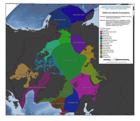
The Arctic Council’s 2009 Arctic Marine Shipping Assessment (AMSA) identified a number of recommendations to guide future action by the Arctic Council, Arctic States and others on current and future Arctic marine activity. Recommendation II C under the theme Protecting Arctic People and the Environment recommended: “That the Arctic states should identify areas of heightened ecological and cultural significance in light of changing climate conditions and increasing multiple marine use and, where appropriate, should encourage implementation of measures to protect these areas from the impacts of Arctic marine shipping, in coordination with all stakeholders and consistent with international law.” As a follow-up to the AMSA, the Arctic Council’s Arctic Monitoring and Assessment Programme (AMAP) and Conservation of Arctic Flora and Fauna (CAFF) working groups undertook to identify areas of heightened ecological significance, and the Sustainable Development Working Group (SDWG) undertook to identify areas of heightened cultural significance. The work to identify areas of heightened ecological significance builds on work conducted during the preparation of the AMAP (2007) Arctic Oil and Gas Assessment. Although it was initially intended that the identification of areas of heightened ecological and cultural significance would be addressed in a similar fashion, this proved difficult. The information available on areas of heightened cultural significance was inconsistent across the Arctic and contained gaps in data quality and coverage which could not be addressed within the framework of this assessment. The areas of heightened cultural significance are therefore addressed within a separate section of the report (Part B) and are not integrated with the information on areas of heightened ecological significance (Part A). In addition, Part B should be seen as instructive in that it illustrates where additional data collection and integration efforts are required, and therefore helps inform future efforts on identification of areas of heightened cultural significance. The results of this work provide the scientific basis for consideration of protective measures by Arctic states in accordance with AMSA recommendation IIc, including the need for specially designated Arctic marine areas as follow-up to AMSA recommendation IId. Reference: AMAP/CAFF/SDWG, 2013. Identification of Arctic marine areas of heightened ecological and cultural significance: Arctic Marine Shipping Assessment (AMSA) IIc. Arctic Monitoring and Assessment Programme (AMAP), Oslo. 114 pp. Data avaiable from: source: <a href="http://www.amap.no/documents/doc/Identification-of-Arctic-marine-areas-of-heightened-ecological-and-cultural-significance-Arctic-Marine-Shipping-Assessment-AMSA-IIc/869" target="_blank">Identification of Arctic marine areas of heightened ecological and cultural significance</a>
-
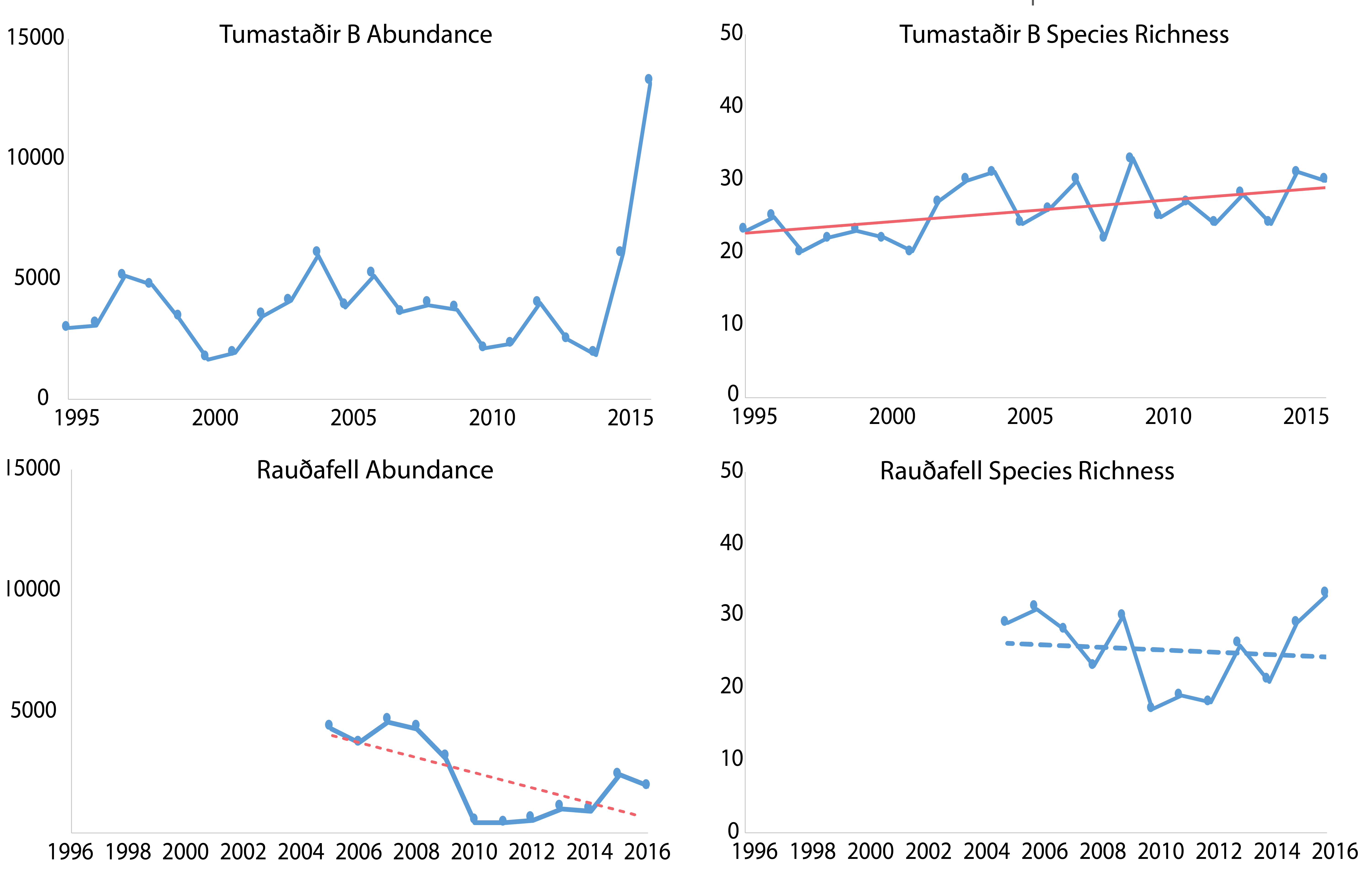
Trends in total abundance of moths and species richness, from two locations in Iceland, 1995–2016. Trends differ between locations. The solid and dashed straight lines represent linear regression lines which are significant or non-significant, respectively. Modified from Gillespie et al. 2020a. STATE OF THE ARCTIC TERRESTRIAL BIODIVERSITY REPORT - Chapter 3 - Page 41 - Figure 3.14
-
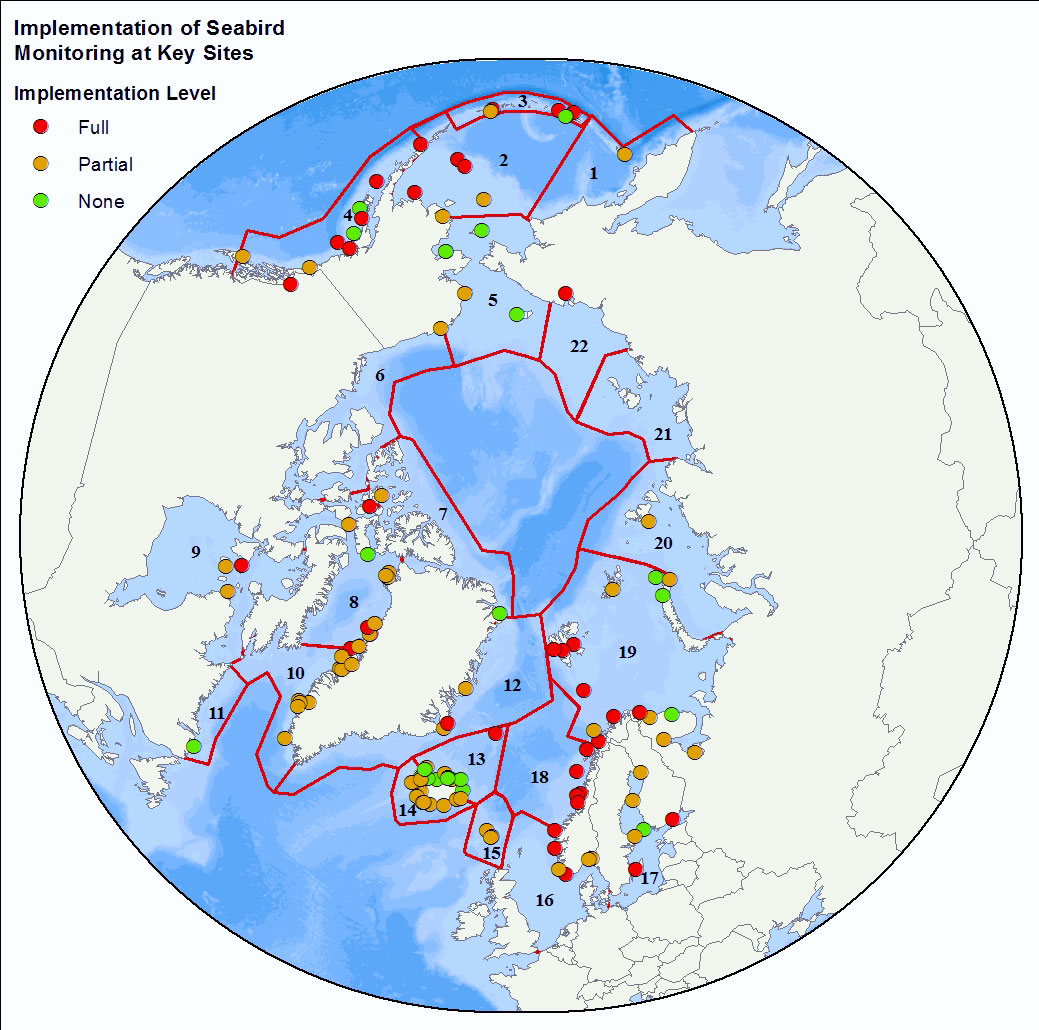
<img width="80px" height="67px" alt="logo" align="left" hspace="10px" src="http://geo.abds.is/geonetwork/srv/eng//resources.get?uuid=7d8986b1-fbd1-4e1a-a7c8-a4cef13e8eca&fname=cbird.png">The Circumpolar Seabird Monitoring Plan is designed to 1) monitor populations of selected Arctic seabird species, in one or more Arctic countries; 2) monitor, as appropriate, survival, diets, breeding phenology, and productivity of seabirds in a manner that allows changes to be detected; 3) provide circumpolar information on the status of seabirds to the management agencies of Arctic countries, in order to broaden their knowledge beyond the boundaries of their country thereby allowing management decisions to be made based on the best available information; 4) inform the public through outreach mechanisms as appropriate; 5) provide information on changes in the marine ecosystem by using seabirds as indicators; and 6) quickly identify areas or issue in the Arctic ecosystem such as declining biodiversity or environmental pressures to target further research and plan management and conservation measures. - <a href="http://caff.is" target="_blank"> Circumpolar Seabird Monitoring plan </a>
-
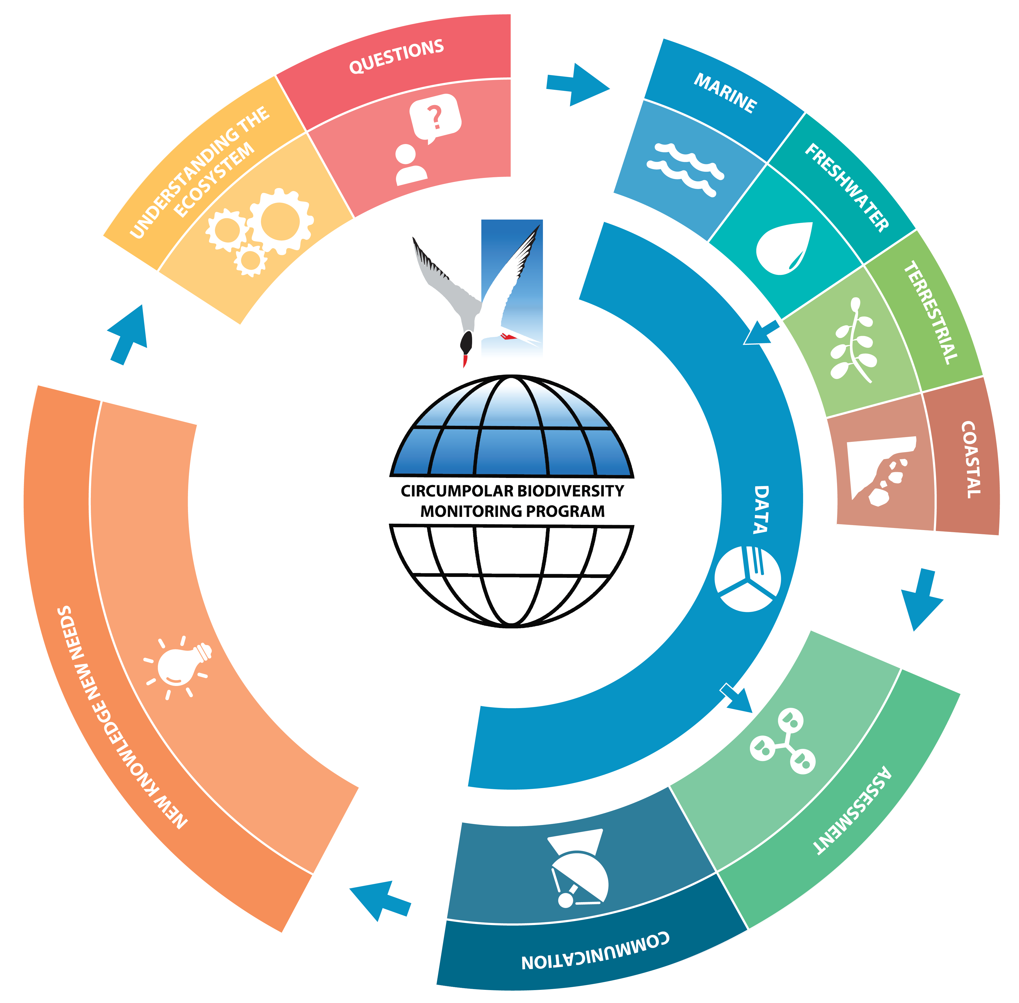
Figure 1-1. CBMP’s adaptive, integrated ecosystem–based approach to inventory, monitoring and data management. This figure illustrates how management questions, conceptual ecosystem models based on science, Indigenous Knowledge, and Local Knowledge, and existing monitoring networks guide the four CBMP monitoring plans––marine, freshwater, terrestrial and coastal. Monitoring outputs (data) feed into the assessment and decision-making processes and guide refinement of the monitoring programmes themselves. Modified from CAFF 2017 STATE OF THE ARCTIC TERRESTRIAL BIODIVERSITY REPORT - Chapter 1 - Page 4 - Figure 1-1
-
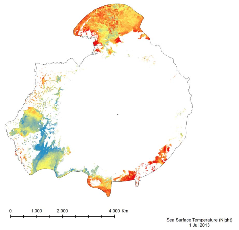
The MODIS Sea Surface Temperature (SST) product provided is a 4km spatialresolution monthly composite made from nighttime measurements from the Aqua Satellite.The nighttime measurements are used to collect a consistent temperature measurement that isunaffected by the warming of the top layer of water by the sun.
-
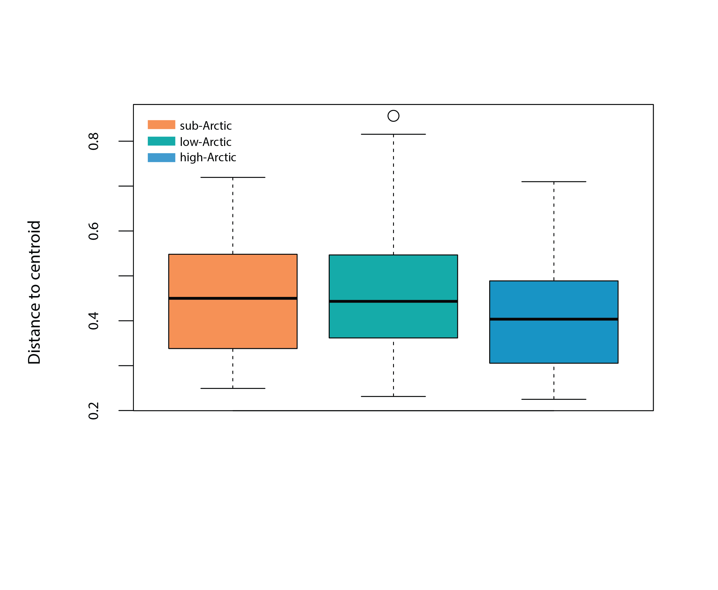
Box plot represents the homogeneity of assemblages in high Arctic (n=190), low Arctic (n=370) and sub-Arctic lakes (n=1151), i.e., the distance of individual lake phytoplankton assemblages to the group centroid in multivariate space. The mean distance to the centroid for each of the regions can be seen as an estimated of beta diversity, with increasing distance equating to greater differences among assemblages. State of the Arctic Freshwater Biodiversity Report - Chapter 4 - Page 48 - Figure 4-18
-
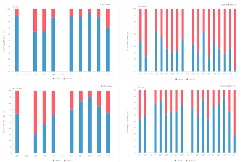
Time series of relative proportions of Arctic and Atlantic Calanus species in Kongsfjorden (top) and Rijpfjorden (bottom) (Source: MOSJ, Norwegian Polar Institute). STATE OF THE ARCTIC MARINE BIODIVERSITY REPORT - <a href="https://arcticbiodiversity.is/findings/plankton" target="_blank">Chapter 3</a> - Page 77 - Figure 3.2.8
-
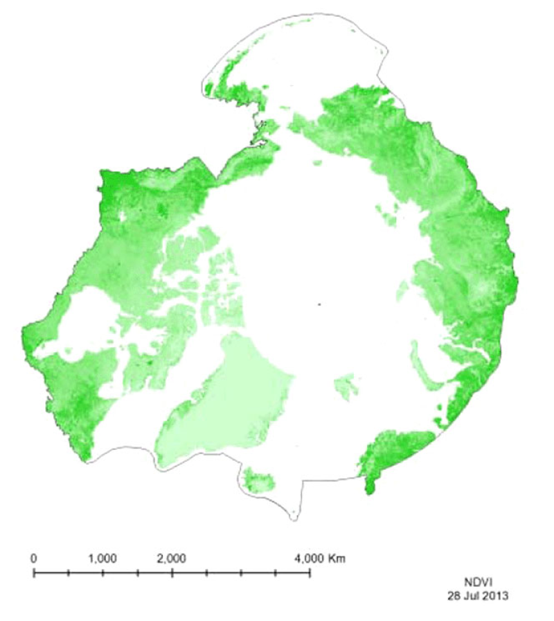
Vegetation indices quantify the concentrations of green leaf vegetation (chlorophyll)around the globe, in an attempt to monitor and correlate vegetation health and stress. The MODIS vegetation products include the Normalized Difference Vegetation Index (NDVI)and an Enhanced Vegetation Index (EVI). Included in the MOD13C1 product is both NDVIand EVI, so both have been provided for the CAFF Dedicated Pan-Arctic Satellite RemoteSensing Products and Distribution System. These indices come in a variety of resolutions,but MTRI has provided a monthly global composite on a 0.05° Climate Model GRID(CMG).
-
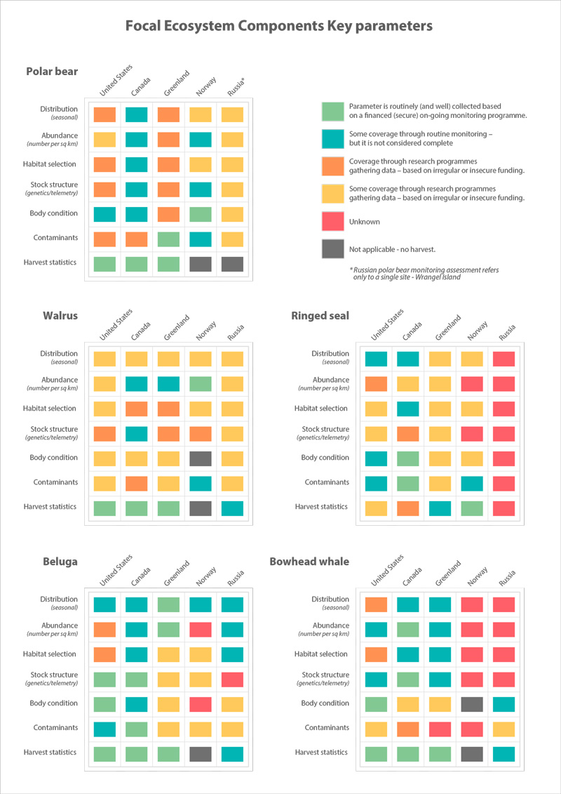
Assessment of monitoring implementation STATE OF THE ARCTIC MARINE BIODIVERSITY REPORT - <a href="https://arcticbiodiversity.is/findings/marine-mammals" target="_blank">Chapter 3</a> - Page 168 - Table 3.6.2
-
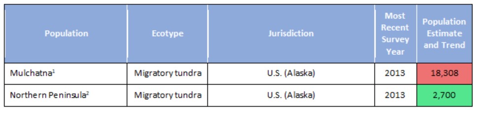
Population estimates and trends for Rangifer populations of the migratory tundra, Arctic island, mountain, and forest ecotypes where their circumpolar distribution intersects the CAFF boundary. Population trends (Increasing, Stable, Decreasing, or Unknown) are indicated by shading. Data sources for each population are indicated as footnotes. STATE OF THE ARCTIC TERRESTRIAL BIODIVERSITY REPORT - Chapter 3 - Page 70 - Table 3.4