 CAFF - Arctic Biodiversity Data Service (ABDS)
dataset
Type of resources
Available actions
Topics
Keywords
Contact for the resource
Provided by
Years
Formats
Representation types
Update frequencies
status
Scale
-
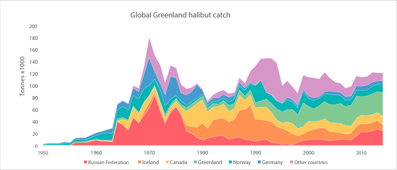
Global catches of Greenland halibut (FAO 2015). STATE OF THE ARCTIC MARINE BIODIVERSITY REPORT - <a href="https://arcticbiodiversity.is/findings/marine-fishes" target="_blank">Chapter 3</a> - Page 121 - Figure 3.4.8
-
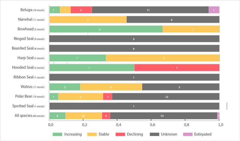
Trends in abundance of Arctic marine mammal Focal Ecosystem Components based on the most recent assessment for each recognized subpopulation of a species (red, declining trend; yellow, stable trend; green, increasing trend; grey, unknown trend). Number of subpopulations is given after species name. Each column is divided into equal segments, the sizes of which are not proportional to the size of the subpopulation. Ringed seal and bearded seal segments represent subspecies. Walrus segments represent subpopulations within subspecies. See Table 3.6.1 for details on abundance. STATE OF THE ARCTIC MARINE BIODIVERSITY REPORT - <a href="https://arcticbiodiversity.is/findings/marine-mammals" target="_blank">Chapter 3</a> - Page 156 - Figure 3.6.2
-
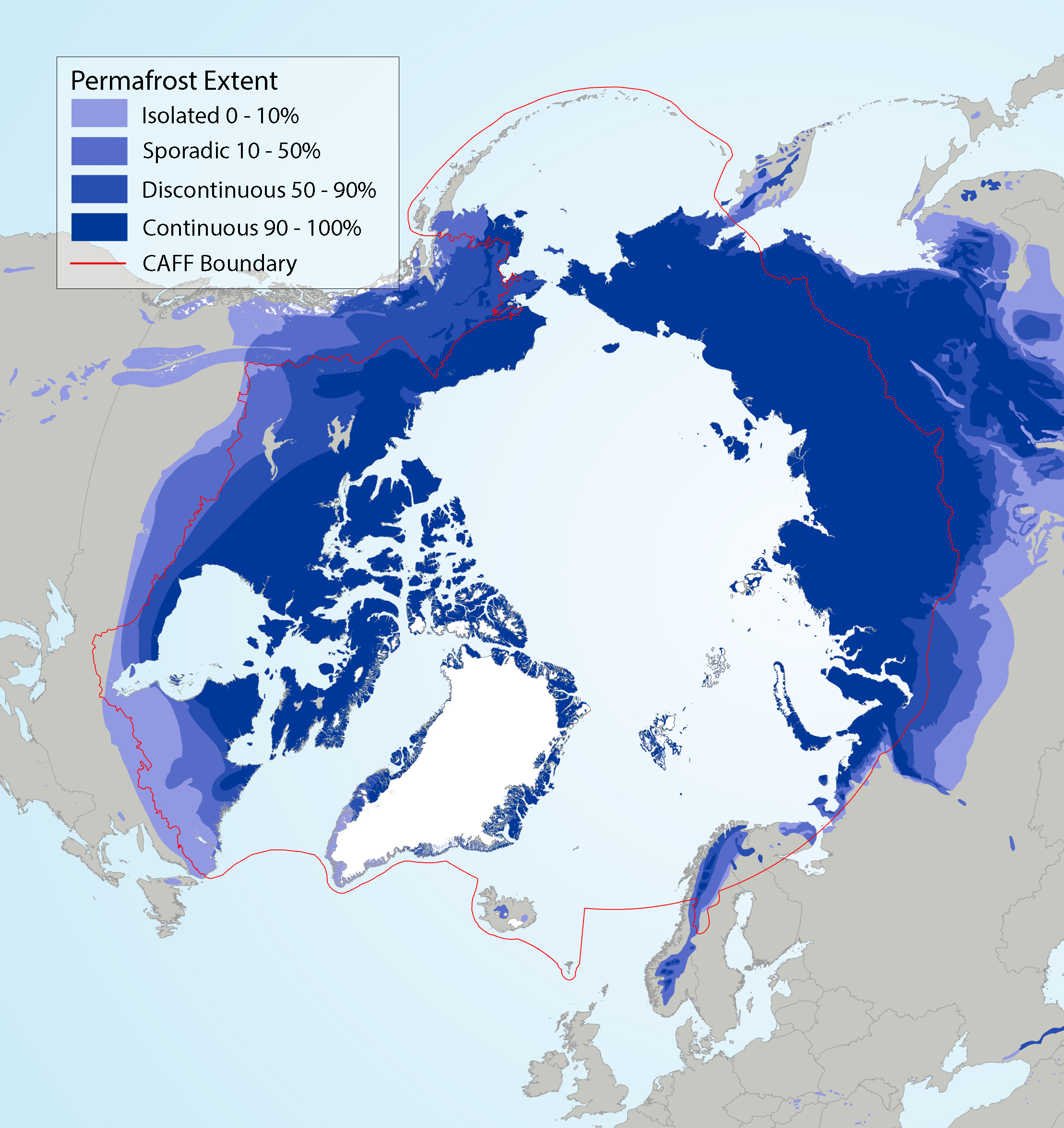
Circumpolar permafrost extent overlain on ecoregions used in SAFBR analysis, indicating continuous (90-100%), discontinuous (50-90%), sporadic (10-50%), and isolated (0-10%) permafrost extent. Source for permafrost layer: Brown et al. (2002). State of the Arctic Freshwater Biodiversity Report - Chapter 5 - Page 89 - Figure 5-6
-
Long-term monitoring programs on benthic fauna are missing for large areas of the Arctic. In areas where repeated monitoring has occurred, it is difficult to compare data due to different sampling approaches and different targets of monitoring efforts. There is a need for an international standardization of long- term benthic monitoring. The CBMP Benthos Expert Network has identified potential ways to improve benthic monitoring coverage, and has come up with a map showing a Pan Arctic station map.
-
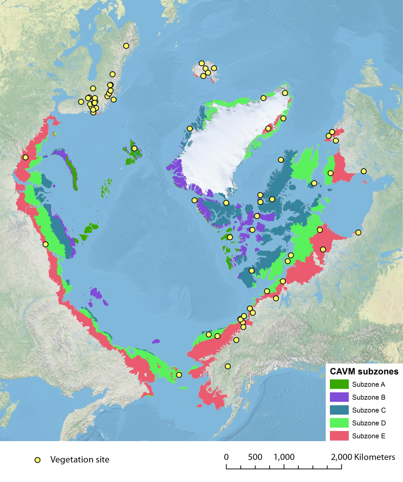
Location of long-term vegetation (including fungi, non-vascular and vascular plants) monitoring sites and programs. Comes from the Arctic Terrestrial Biodiversity Monitoring Plan is developed to improve the collective ability of Arctic traditional knowledge holders, northern communities and scientists to detect, understand and report on long-term change in Arctic terrestrial ecosystems and biodiversity. The report can be seen here http://www.caff.is/publications/view_document/256-arctic-terrestrial-biodiversity-monitoring-plan The monitoring locations are place over the Circumpolar Arctic bioclimate subzones (CAVM Team 2003) http://www.caff.is/flora-cfg/circumpolar-arctic-vegetation-map
-
Critical to the successful implementation of EBM in the Arctic is the existence of a cohesive circumpolar approach to the collection and management of data and the application of compatible frameworks, standards and protocols that this entails. STATE OF THE ARCTIC MARINE BIODIVERSITY REPORT - <a href="https://arcticbiodiversity.is/marine" target="_blank">Chapter 2</a> - Page 29 - Box Figure 2.2
-
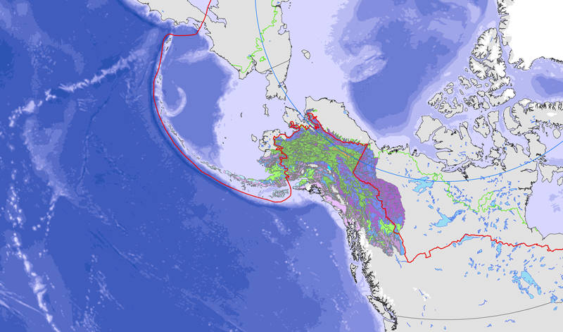
<a href="http://caff.is/strategies-series/359-the-alaska-yukon-region-of-the-circumboreal-vegetation-map-cbvm" target="_blank"> <img width="150px" height="150px" alt="logo" align="left" hspace="10px" src="http://geo.abds.is/geonetwork/images/flora_logo.png"> </a>A map of boreal vegetation for the Alaska-Yukon region was developed to contribute to the circumboreal vegetation mapping (CBVM) project. The effort included developing a map of bioclimates with 12 bioclimate zones, a map of biogeographic provinces with Alaska-Yukon and Aleutian provinces, and a map of geographic sectors with six sectors that provided the basis for classification of boreal vegetation. Vegetation mapping was done at 1:7.5 million scale using the mapping protocols of the CBVM team. Mapping used MODIS imagery as the basis for manual image interpretation and an integrated-terrain-unit approach, which included classifications for bioclimate, physiography, generalized geology, permafrost, disturbance, growth from, geographic sector, and vegetation. Vegetation was mapped at two hierarchical levels: (1) formation group differentiating zonal and azonal systems; and (2) geographic sectors based on bioclimatic zonation and dominant species that characterize broad longitudinal regions or biogeographic provinces. Each of the 19 map units was described by identifying the dominant and characteristic species and its climatic and landscape characteristics, as well as references that relate to the unit.
-
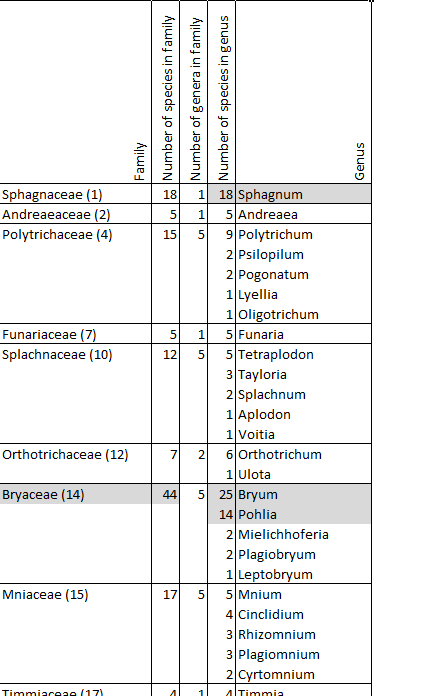
Appendix 9.8 The thirty moss families of the Canadian Arctic Archipelago with reference number (Ireland et al. 1987) in brackets. Number of species in each family, number of genus in family, and number of species in each genus are given. Species-rich genera and families are highlighted in grey.
-
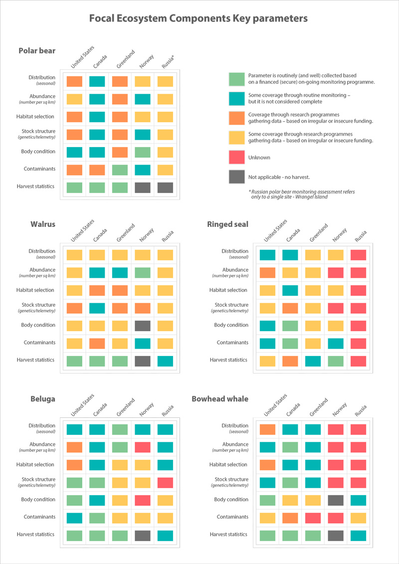
Assessment of monitoring implementation STATE OF THE ARCTIC MARINE BIODIVERSITY REPORT - <a href="https://arcticbiodiversity.is/findings/marine-mammals" target="_blank">Chapter 3</a> - Page 168 - Table 3.6.2
-
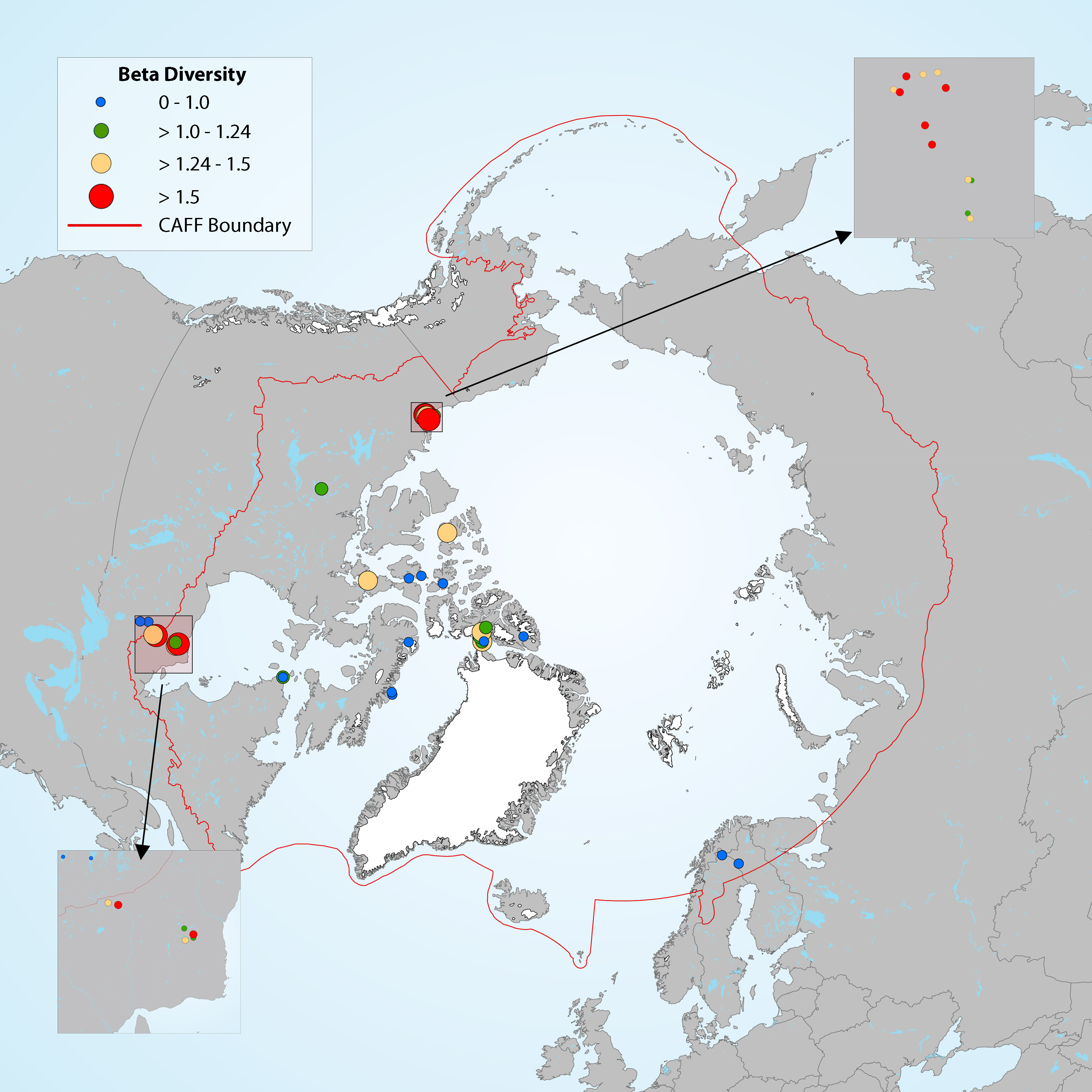
Figure 4-16 Map showing the magnitude of change in diatom assemblages for downcore samples, with beta diversity used as a measure of the compositional differences between samples at different depths along the core. Boundaries for the beta diversity categories are based on distribution quartiles (0-0.1, 0.1-1.24, 1.24-1.5, >1.5), where the lowest values (blue dots) represent the lowest degree of change in diatom assemblage composition along the length of the core in each lake. State of the Arctic Freshwater Biodiversity Report - Chapter 2 - Page 15 - Figure 2-1