 CAFF - Arctic Biodiversity Data Service (ABDS)
Marine
Type of resources
Available actions
Topics
Keywords
Contact for the resource
Provided by
Years
Formats
Representation types
Update frequencies
status
Scale
-
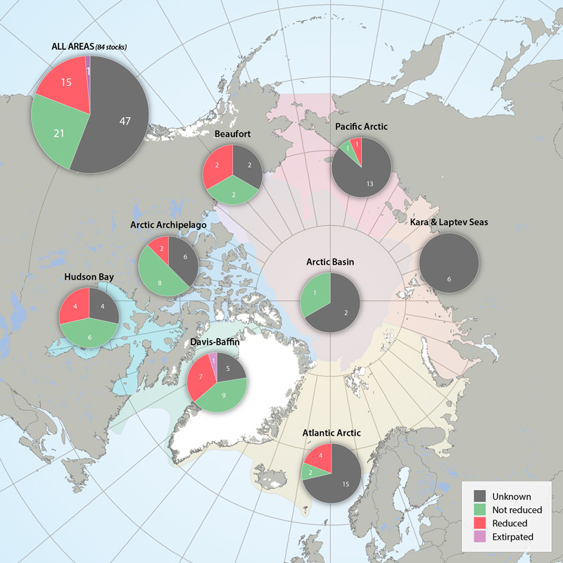
Status of marine mammal Focal Ecosystem Component stocks by Arctic Marine Area. STATE OF THE ARCTIC MARINE BIODIVERSITY REPORT - <a href="https://arcticbiodiversity.is/findings/marine-mammals" target="_blank">Chapter 3</a> - Page 157 - Figure 3.6.3
-
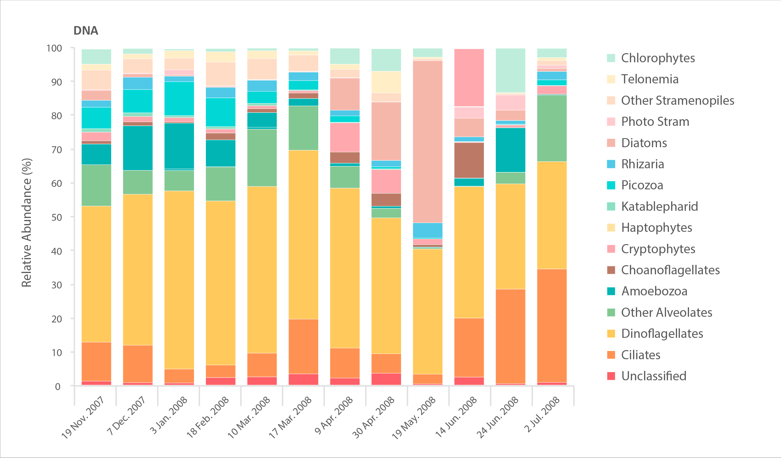
Relative abundance of major eukaryote taxonomic groups found by high throughput sequencing of the small-subunit (18S) rRNA gene. Time series collected by sampling every 2-6 weeks in Amundsen Gulf of the Beaufort Sea over the winter-spring transition in 2007–2008. Sampling DNA gives information about presence/absence, while sampling RNA gives information about the state of activity of different taxa. STATE OF THE ARCTIC MARINE BIODIVERSITY REPORT - <a href="https://arcticbiodiversity.is/findings/plankton" target="_blank">Chapter 3</a> - Page 72 - Figures 3.2.3
-
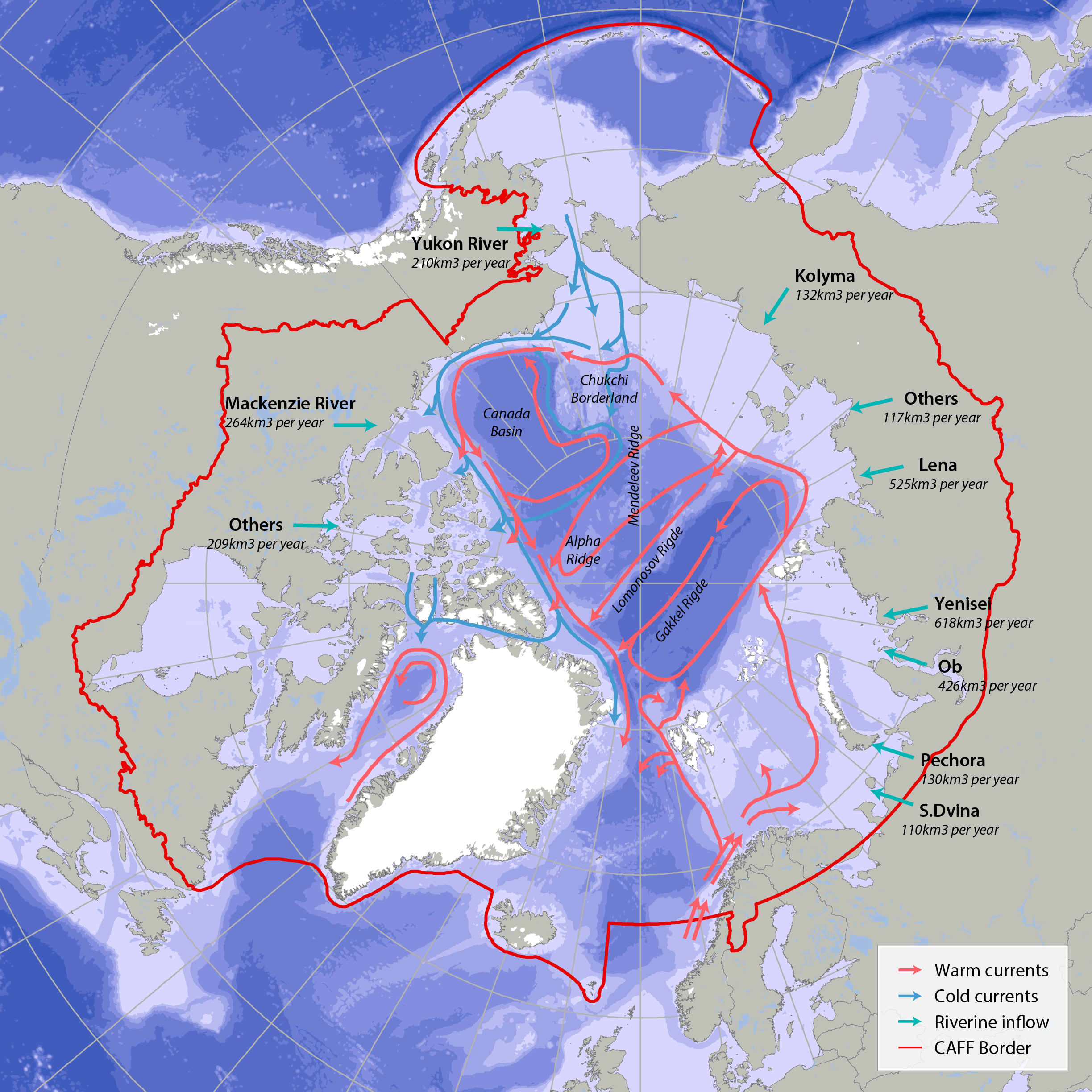
Bathymetric features, warm currents (red arrows), cold currents (blue arrows) and riverine inflow in the Arctic. Adapted from Jakobsen et al. (2012). Simplified Arctic Ocean currents (Fig. 2.1) show that the main circulation patterns follow the continental shelf breaks and margins of the basins in the Arctic Ocean. Different global models predict different types of changes, which can cause changes to Arctic ecosystems (AMAP 2013, Meltofte 2013). STATE OF THE ARCTIC MARINE BIODIVERSITY REPORT - <a href="https://arcticbiodiversity.is/marine" target="_blank">Chapter 2</a> - Page 22 - Figure 2.1
-
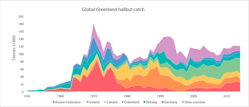
Global catches of Greenland halibut (FAO 2015). STATE OF THE ARCTIC MARINE BIODIVERSITY REPORT - <a href="https://arcticbiodiversity.is/findings/marine-fishes" target="_blank">Chapter 3</a> - Page 121 - Figure 3.4.8
-
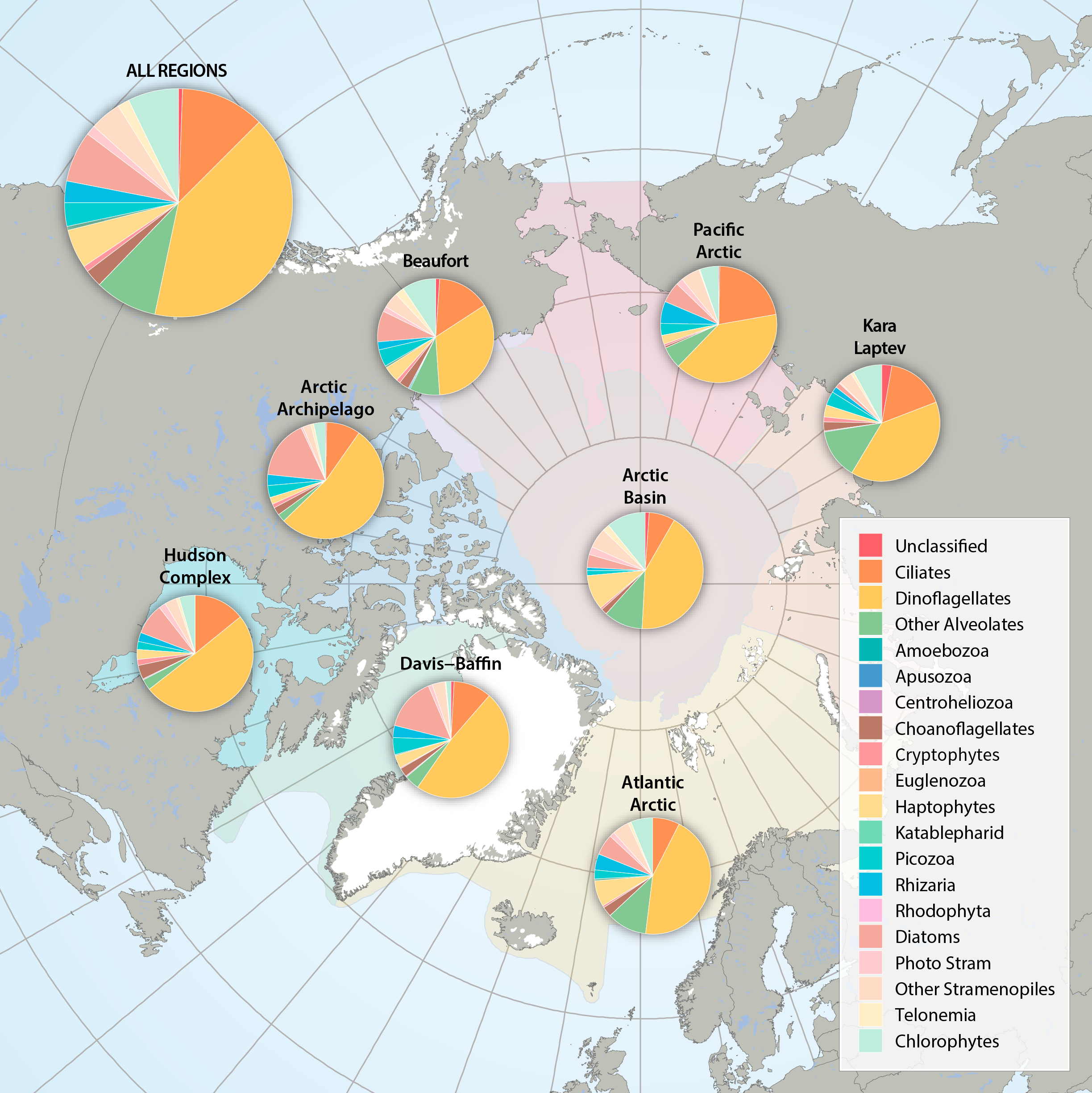
Figure 3.2.2a: Relative abundance of major eukaryote taxonomic groups found by high throughput sequencing of the small-subunit (18S) rRNA gene across Arctic Marine Areas. Figure 3.2.2b: Relative abundance of major eukaryote functional groups found by microscopy in the Arctic Marine Areas. STATE OF THE ARCTIC MARINE BIODIVERSITY REPORT - <a href="https://arcticbiodiversity.is/findings/plankton" target="_blank">Chapter 3</a> - Page 70 - Figures 3.2.2a and 3.2.2b
-
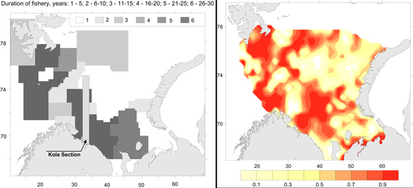
Commercial fishery impact on zoobenthos of the Barents Sea. Figure A) Intensity and duration of fishery efforts in standard commercial fishery areas in the Barents Sea. The darker the area the longer the fishery has been in operation. Figure B) Level of decline in macrobenthic biomass between 1926-1932 and 1968-1970 calculated as 1-b1968/b1930. The largest biomass decreases correspond to the darker colour, whereas lighter colour refers to no change (Denisenko 2013). STATE OF THE ARCTIC MARINE BIODIVERSITY REPORT - <a href="https://arcticbiodiversity.is/findings/benthos" target="_blank">Chapter 3</a> - Page 97 - Figure 3.3.4
-
Critical to the successful implementation of EBM in the Arctic is the existence of a cohesive circumpolar approach to the collection and management of data and the application of compatible frameworks, standards and protocols that this entails. STATE OF THE ARCTIC MARINE BIODIVERSITY REPORT - <a href="https://arcticbiodiversity.is/marine" target="_blank">Chapter 2</a> - Page 29 - Box Figure 2.2
-
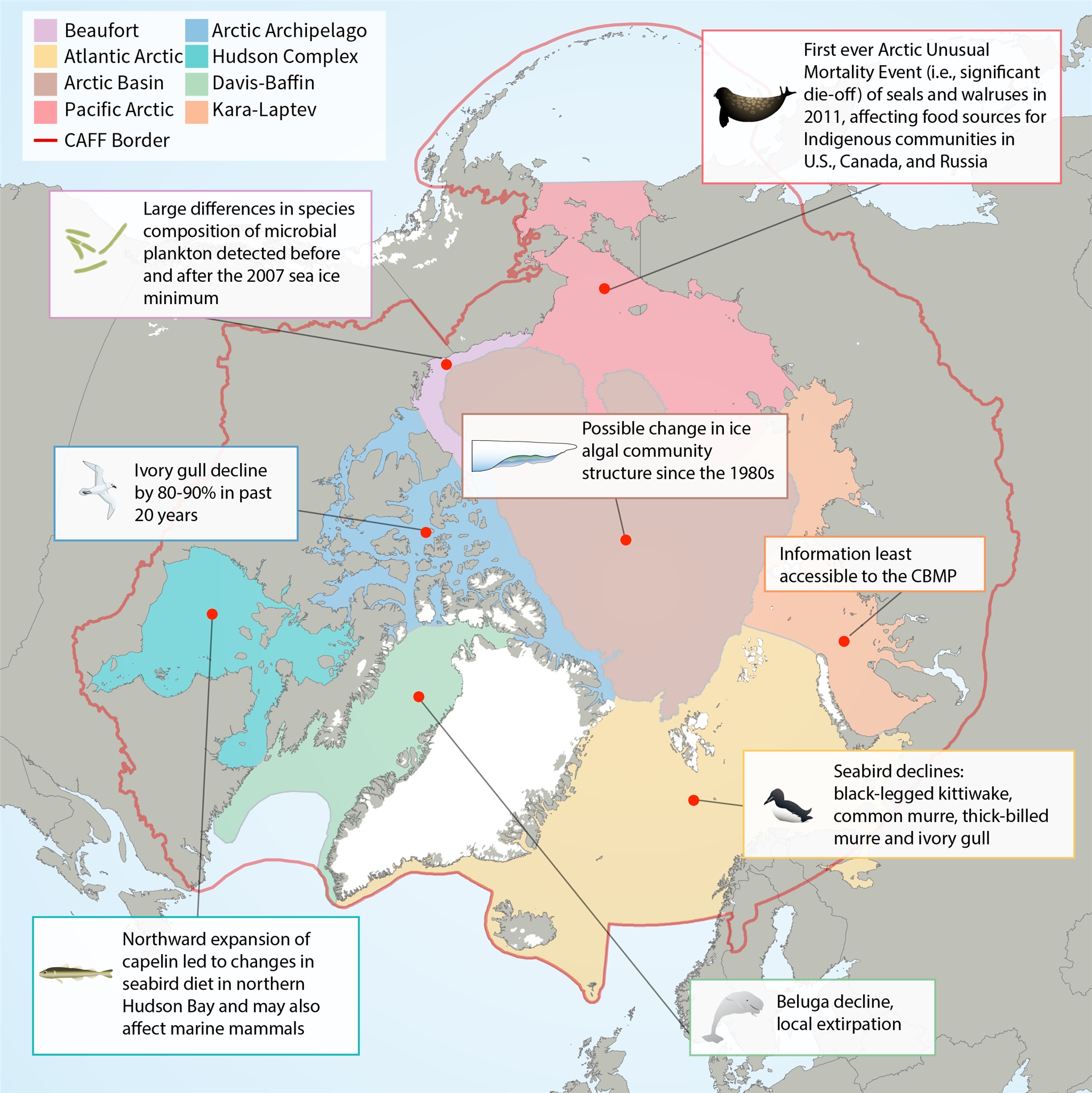
Map of Arctic Marine Areas as defined by the Circumpolar Biodiversity Monitoring Program (CBMP), with one sample finding from each area.
-
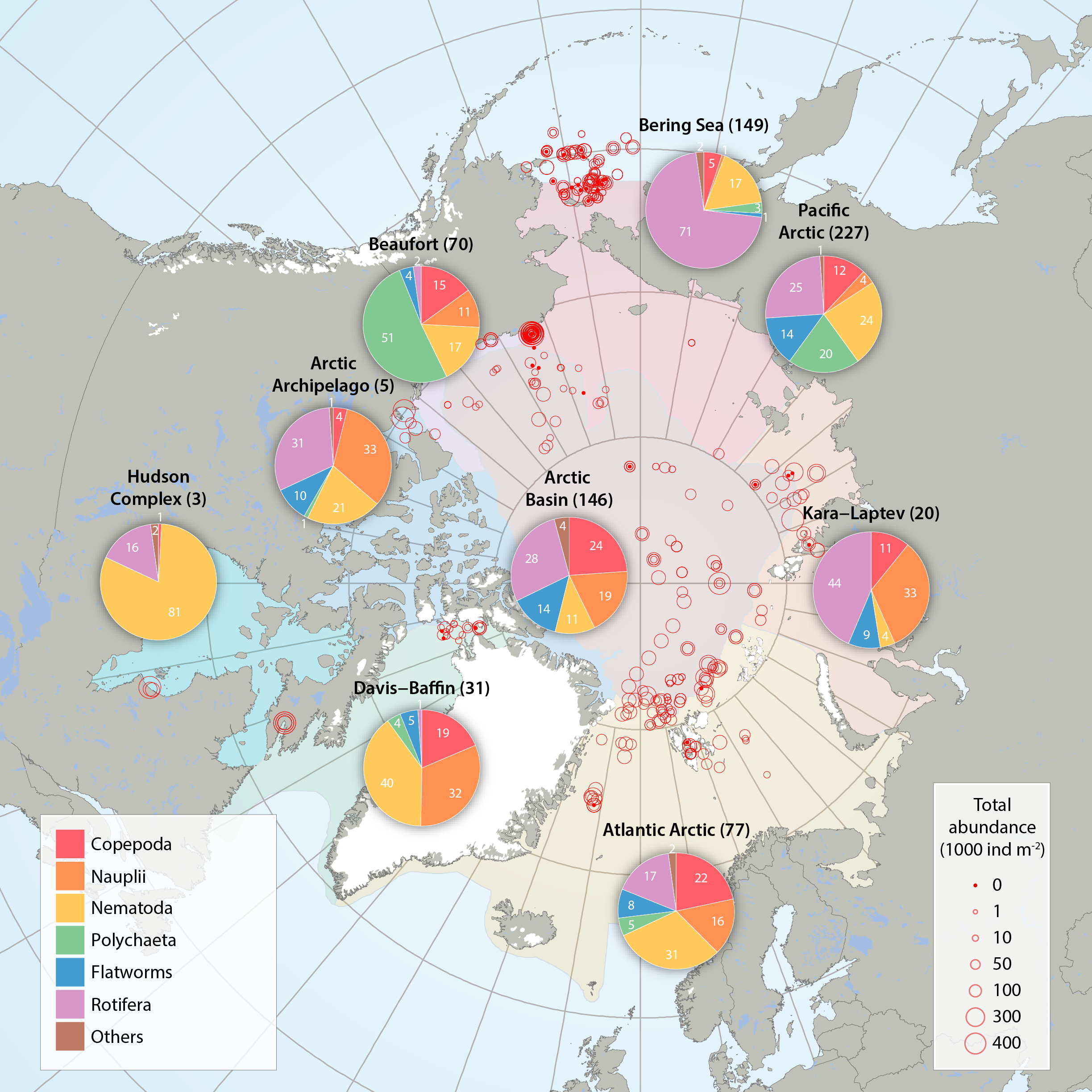
Sea ice meiofauna composition (pie charts) and total abundance (red circles) across the Arctic, compiled by the CBMP Sea Ice Biota Expert Network from 27 studies between 1979 and 2015. Scaled circles show total abundance per individual ice core while pie charts show average relative contribution by taxon per Arctic Marine Area (AMA). Number of ice cores for each AMA is given in parenthesis after region name. Note that studies were conducted at different times of the year, with the majority between March and August (see 3.1 Appendix). The category ‘other’ includes young stages of bristle worms (Polychaeta), mussel shrimps (Ostracoda), forams (Foraminifera), hydroid polyps (Cnidaria), comb jellies (Ctenophora), sea butterflies (Pteropoda), marine mites (Acari) and unidentified organisms. STATE OF THE ARCTIC MARINE BIODIVERSITY REPORT - <a href="https://arcticbiodiversity.is/findings/sea-ice-biota" target="_blank">Chapter 3</a> - Page 40 - Figure 3.1.4 From the report draft: "Here, we synthesized 19 studies across the Arctic conducted between 1979 and 2015, including unpublished sources (B. Bluhm, R. Gradinger, UiT – The Arctic University of Norway; H. Hop, Norwegian Polar Institute; K. Iken, University of Alaska Fairbanks). These studies sampled landfast sea ice and offshore pack ice, both first- and multiyear ice (Appendix 3.1). Meiofauna abundances reported in individual data sources were converted to individuals m-2 of sea ice assuming that ice density was 95% of that in melted ice. Due to the low taxonomic resolution in the reviewed studies, ice meiofauna were grouped into: Copepoda, nauplii (for copepods as well as other taxa with naupliar stages), Nematoda, Polychaeta (mostly juveniles, but also trochophores), flatworms (Acoelomorpha and Platyhelminthes; these phyla have mostly been reported as one category), Rotifera, and others (which include meroplanktonic larvae other than Polychaeta, Ostracoda, Foraminifera, Cnidaria, Ctenophora, Pteropoda, Acari, and unidentified organisms). Percentage of total abundance for each group was calculated for each ice core, and these percentages were used for regional averages. Maximum available ice core length was used in data analysis, but 50% of these ice cores included only the bottom 10 cm of the ice, 12% the bottom 5 cm, 10% the bottom 2 cm, and 11% the entire ice-thickness. Data from 617 cores were used."
-
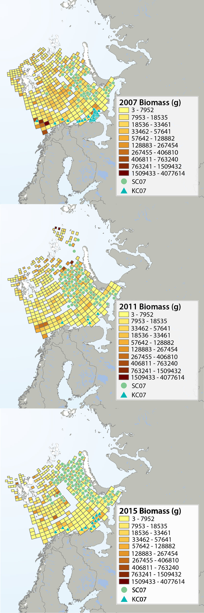
Megafauna distribution of biomass (g/15 min trawling) in the Barents Sea in 2007, 2011 and 2015. The green circles show the distribution of the snow crab as it spreads from east to west, and the blue triangles show the invasion of king crab along the coast of the southern Barents Sea. Data from Institute of Marine Research, Norway and the Polar Research Institute of Marine Fisheries and Oceanography, Murmansk, Russia. STATE OF THE ARCTIC MARINE BIODIVERSITY REPORT - <a href="https://arcticbiodiversity.is/findings/benthos" target="_blank">Chapter 3</a> - Page 95 - Figure 3.3.2 The annual joint Norwegian–Russian Ecosystem Survey provides from more than 400 stations and during extensive cruise tracks covering more or less the whole Barents Sea in August– September. The sampling is based on a regular grid spanning about 1.5 millionkm2 with fixed positions of stations which make it possible to measure changes in spatial distribution over time. The trawl is a Campelen 1800 bottom trawl rigged with rock-hopper groundgear and towed on double Warps. The mesh size is 80 mm (stretched) in the front and 16–22 mmin the cod end, allowing the capture and retention of smaller fish and the largest benthos from the seabed (benthic megafauna). The horizontal opening was 11.7 m, and the vertical opening 4–5 m (Teigsmark and Øynes, 1982). The trawl configuration and bottom contact was monitored remotely by SCANMAR trawl sensors. The standard distance between trawl stations was 35 nautical miles (65 km), except north and west of Svalbard where a stratified sampling was adapted to the steep continental shelve. The standard procedure was to tow 15 min after the trawl had made contact with the bottom, but the actual tow duration ranged between 5 min and 1 h and data were subsequently standardized to 15 min trawl time. Towing speed was 3 knots, equivalent to a towing distance of 0.75 nautical miles (1.4 km) during a 15 min tow. The trawl catches were recorded using the same procedures on the Russian and the Norwegian Research vessels to ensure comparability across Barents Sea regions. The benthic megafauna was separated from the fish and shrimp catch, washed, and sorted to lowest possible taxonomic level, in most cases to species, on-Board the vessel. Species identification was standardized between the researcher teams by annually exchanging the benthic expert’s among the vessels and taxon names were fixed each year according toWORMSwhen possible.This resulted in an Electronic identification manual and photo-compendium as a tool to standardize taxon identifications, in addition to various sources of identification literature. Difficult taxa were photographed and, in some cases, brought back as preserved voucher specimens for further identification. Wet-weight biomass was recorded with electronic scales in the ship laboratories for each taxon.The biomass determination included all fragments.