 CAFF - Arctic Biodiversity Data Service (ABDS)
dataset
Type of resources
Available actions
Topics
Keywords
Contact for the resource
Provided by
Years
Formats
Representation types
Update frequencies
status
Scale
-
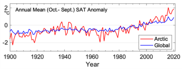
Warming in the Arctic has been significantly faster than anywhere else on Earth (Ballinger et al. 2020). Trends in land surface temperature are shown on Figure 2-2. STATE OF THE ARCTIC TERRESTRIAL BIODIVERSITY REPORT - Chapter 2 - Page 23 - Figure 2.2
-

The Seabird Information Network (SIN) developed by the Circumpolar Seabird expert group (<a href="http://caff.is/seabirds-cbird" target="_blank">CBird</a>) of the Conservation of Arctic Flora and Fauna (<a href="http://caff.is" target="_blank">CAFF</a>) working group of the Arctic Council focuses on the development of a data entry and analysis portal system allowing for circumpolar seabird colony information to be contributed, mapped, and shared by scientists and monitoring programs around the Arctic. - <a href="http://axiom.seabirds.net/maps/js/seabirds.php?app=circumpolar#z=2&ll=NaN,0.00000" target="_blank"> Circumpolar Seabird portal</a>
-
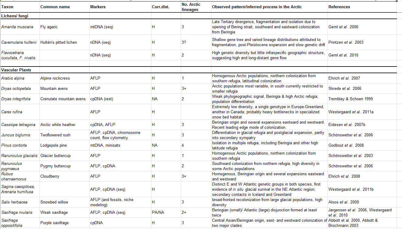
Appendix 17.3. Phylogeographic and population genetics studies of selected Arctic species.
-
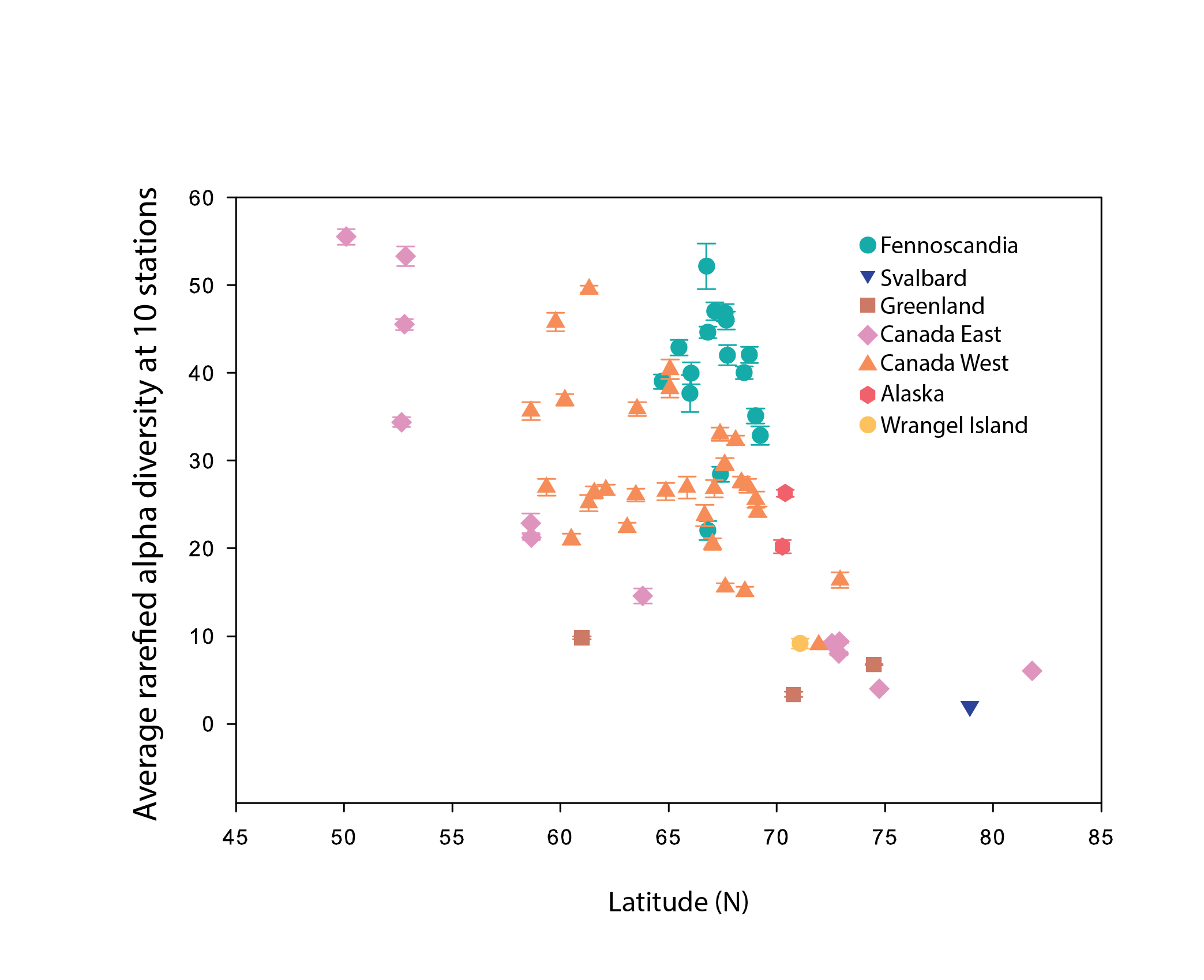
Alpha diversity (rarefied to 10 stations, with error bars indicating standard error) of river benthic macroinvertebrates plotted as a function of the average latitude of stations in each hydrobasin. Hydrobasins are coloured based on country/region State of the Arctic Freshwater Biodiversity Report - Chapter 4 - Page 68 - Figure 4-32
-
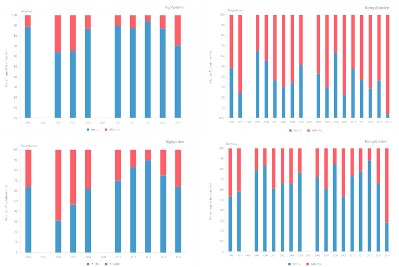
Time series of relative proportions of Arctic and Atlantic Calanus species in Kongsfjorden (top) and Rijpfjorden (bottom) (Source: MOSJ, Norwegian Polar Institute). STATE OF THE ARCTIC MARINE BIODIVERSITY REPORT - <a href="https://arcticbiodiversity.is/findings/plankton" target="_blank">Chapter 3</a> - Page 77 - Figure 3.2.8
-
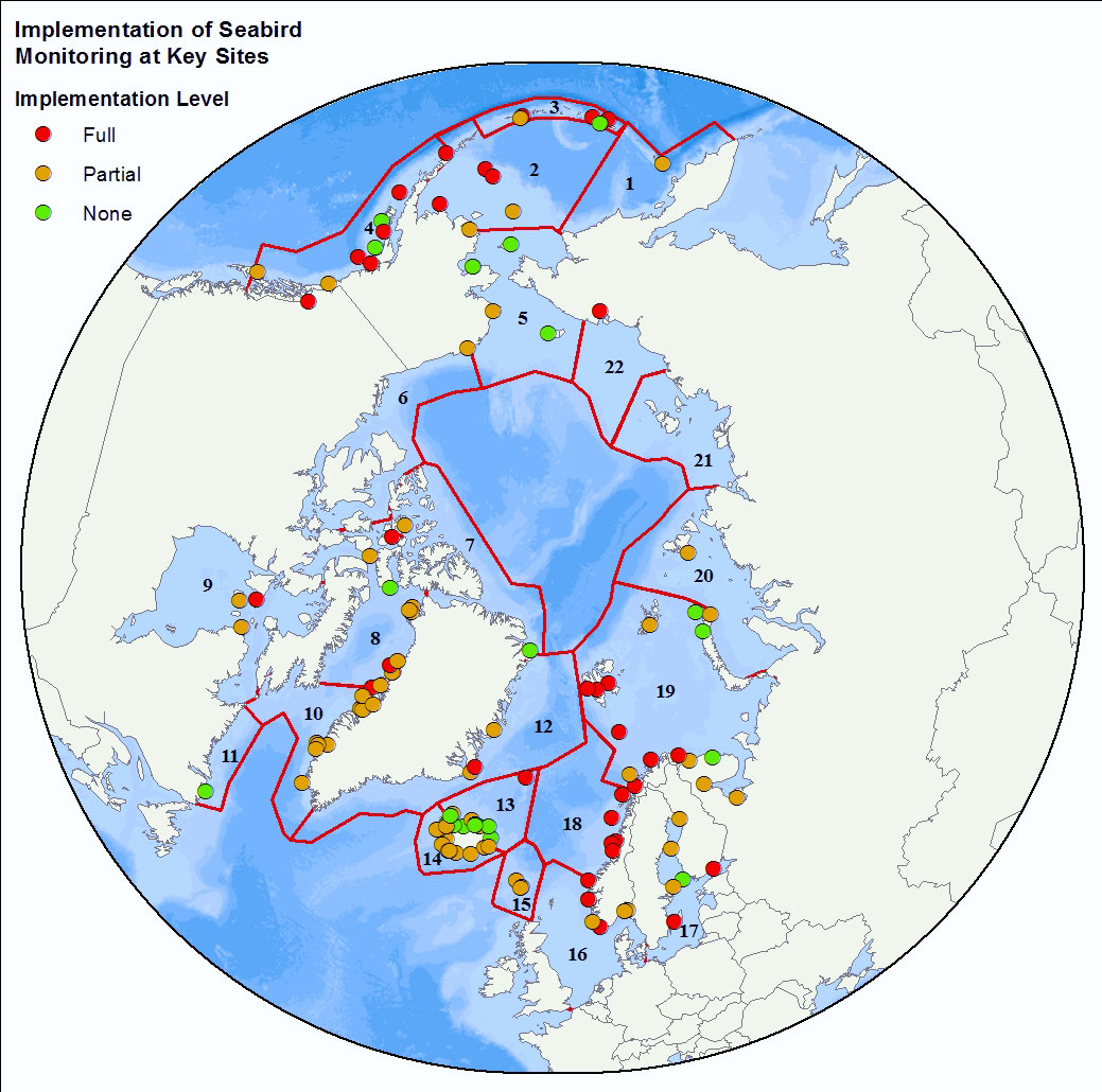
<img width="80px" height="67px" alt="logo" align="left" hspace="10px" src="http://geo.abds.is/geonetwork/srv/eng//resources.get?uuid=7d8986b1-fbd1-4e1a-a7c8-a4cef13e8eca&fname=cbird.png">The Circumpolar Seabird Monitoring Plan is designed to 1) monitor populations of selected Arctic seabird species, in one or more Arctic countries; 2) monitor, as appropriate, survival, diets, breeding phenology, and productivity of seabirds in a manner that allows changes to be detected; 3) provide circumpolar information on the status of seabirds to the management agencies of Arctic countries, in order to broaden their knowledge beyond the boundaries of their country thereby allowing management decisions to be made based on the best available information; 4) inform the public through outreach mechanisms as appropriate; 5) provide information on changes in the marine ecosystem by using seabirds as indicators; and 6) quickly identify areas or issue in the Arctic ecosystem such as declining biodiversity or environmental pressures to target further research and plan management and conservation measures. - <a href="http://caff.is" target="_blank"> Circumpolar Seabird Monitoring plan </a>
-
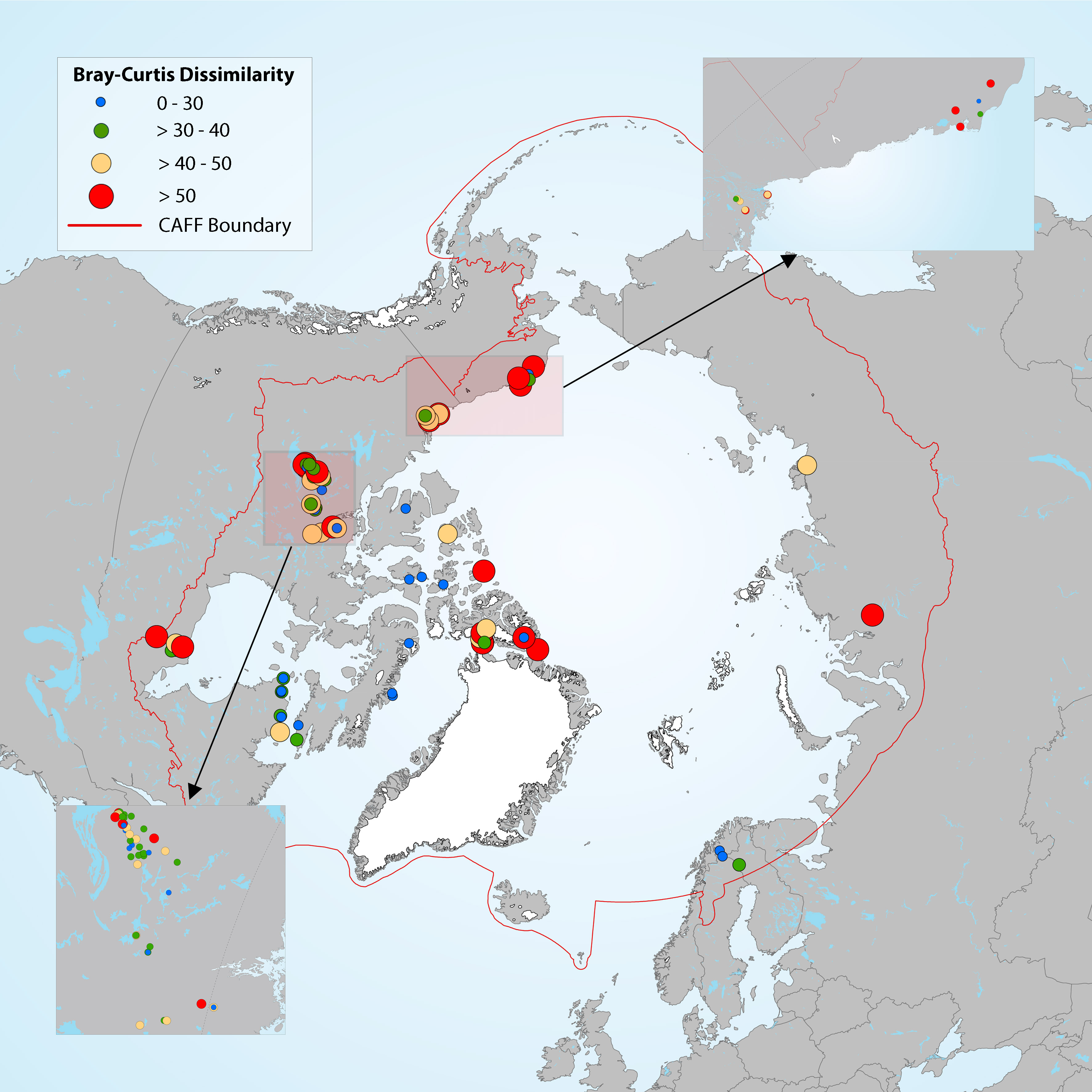
Estimation of diatom assemblage changes over a period of about 200 years (top versus bottom sediment cores). Figure 4-14 Map showing the magnitude of change in diatom assemblages between bottom (pre-industrial) and top (modern) section of the cores, estimated by Bray-Curtis (B-C) dissimilarity. Boundaries for the B-C dissimilarity categories are based on distribution quartiles (0-30%, 30-40%, 40- 50% and >50%), where the lowest values (blue dots) represent the lowest degree of change in diatom assemblage composition between top and bottom sediment core samples in each lake. State of the Arctic Freshwater Biodiversity Report - Chapter 4 - Page 41 - Figure 4-14
-
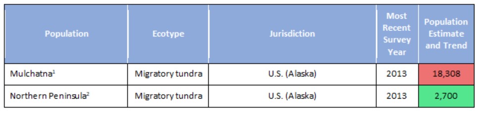
Population estimates and trends for Rangifer populations of the migratory tundra, Arctic island, mountain, and forest ecotypes where their circumpolar distribution intersects the CAFF boundary. Population trends (Increasing, Stable, Decreasing, or Unknown) are indicated by shading. Data sources for each population are indicated as footnotes. STATE OF THE ARCTIC TERRESTRIAL BIODIVERSITY REPORT - Chapter 3 - Page 70 - Table 3.4
-
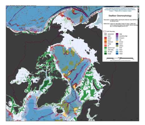
We present the first digital seafloor geomorphic features map (GSFM) of the global ocean. The GSFM includes 131,192 separate polygons in 29 geomorphic feature categories, used here to assess differences between passive and active continental margins as well as between 8 major ocean regions (the Arctic, Indian, North Atlantic, North Pacific, South Atlantic, South Pacific and the Southern Oceans and the Mediterranean and Black Seas). The GSFM provides quantitative assessments of differences between passive and active margins: continental shelf width of passive margins (88 km) is nearly three times that of active margins (31 km); the average width of active slopes (36 km) is less than the average width of passive margin slopes (46 km); active margin slopes contain an area of 3.4 million km2 where the gradient exceeds 5°, compared with 1.3 million km2 on passive margin slopes; the continental rise covers 27 million km2 adjacent to passive margins and less than 2.3 million km2 adjacent to active margins. Examples of specific applications of the GSFM are presented to show that: 1) larger rift valley segments are generally associated with slow-spreading rates and smaller rift valley segments are associated with fast spreading; 2) polar submarine canyons are twice the average size of non-polar canyons and abyssal polar regions exhibit lower seafloor roughness than non-polar regions, expressed as spatially extensive fan, rise and abyssal plain sediment deposits – all of which are attributed here to the effects of continental glaciations; and 3) recognition of seamounts as a separate category of feature from ridges results in a lower estimate of seamount number compared with estimates of previous workers. Reference: Harris PT, Macmillan-Lawler M, Rupp J, Baker EK Geomorphology of the oceans. Marine Geology.
-
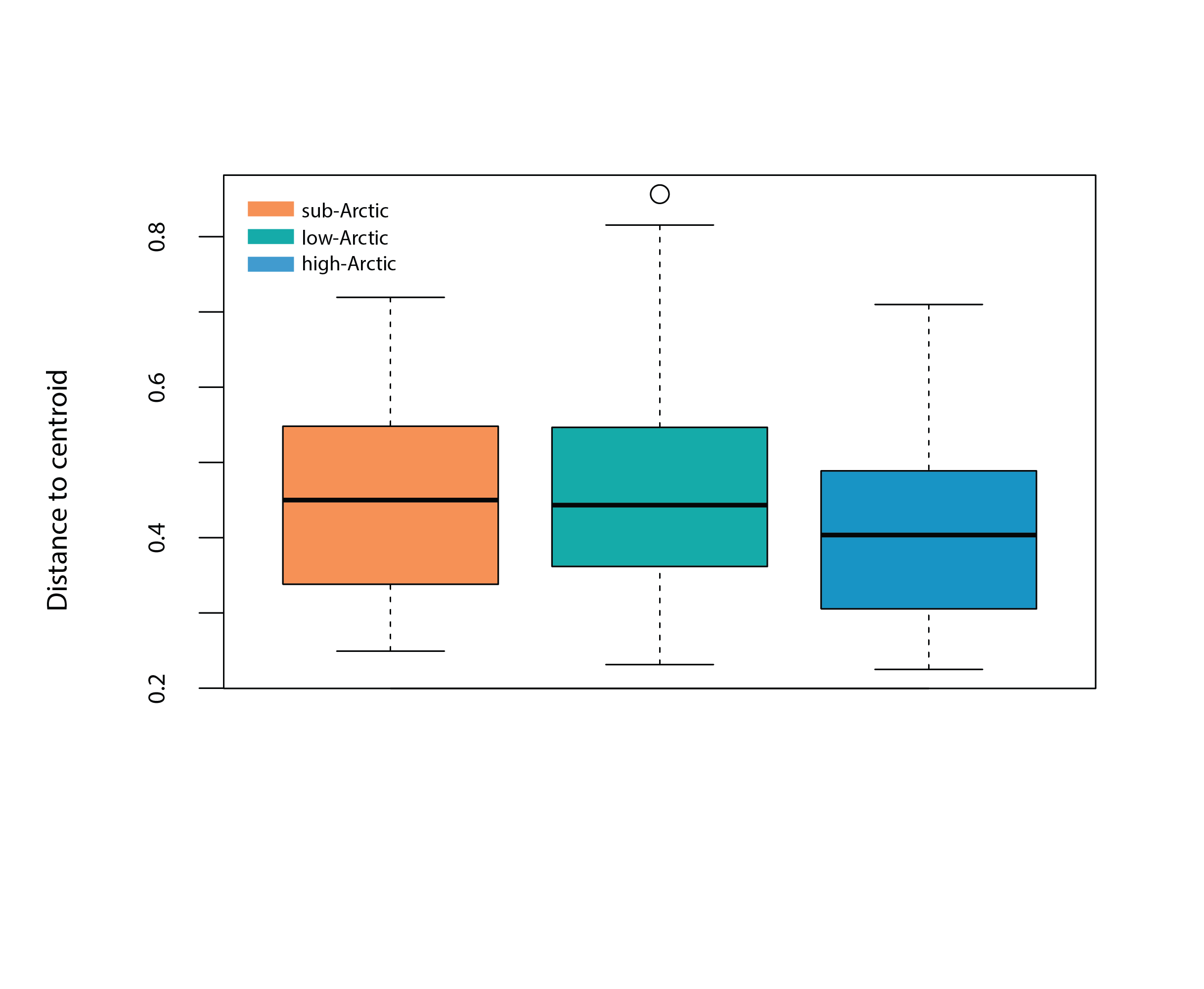
Box plot represents the homogeneity of assemblages in high Arctic (n=190), low Arctic (n=370) and sub-Arctic lakes (n=1151), i.e., the distance of individual lake phytoplankton assemblages to the group centroid in multivariate space. The mean distance to the centroid for each of the regions can be seen as an estimated of beta diversity, with increasing distance equating to greater differences among assemblages. State of the Arctic Freshwater Biodiversity Report - Chapter 4 - Page 48 - Figure 4-18