 CAFF - Arctic Biodiversity Data Service (ABDS)
Type of resources
Available actions
Topics
Keywords
Contact for the resource
Provided by
Years
Formats
Representation types
Update frequencies
status
Service types
Scale
-
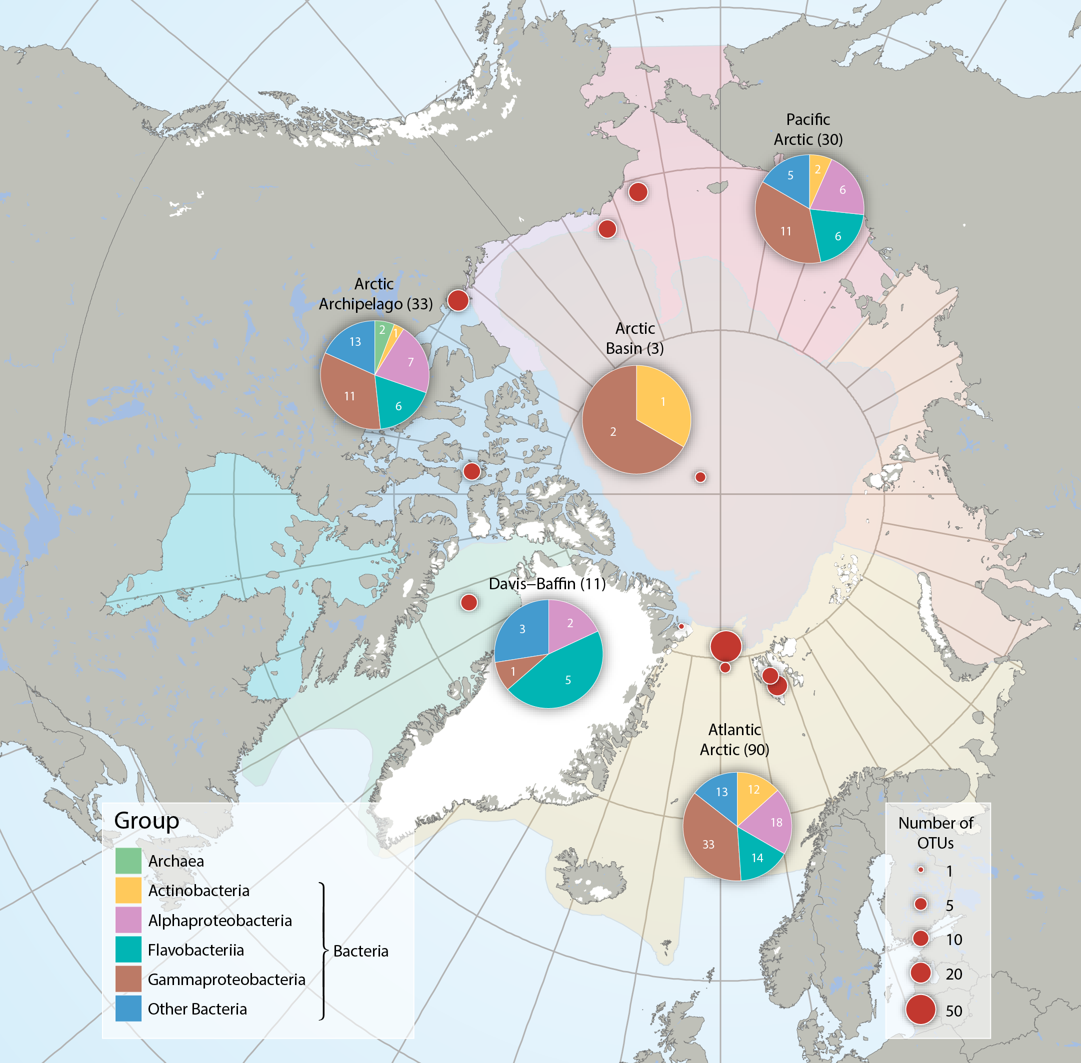
Bacteria and Archaea across five Arctic Marine Areas based on number of operational taxonomic units (OTUs), or molecular species. Composition of microbial groups, with respective numbers of OTUs (pie charts) and number of OTUs at sampling locations (red dots). Data aggregated by the CBMP Sea Ice Biota Expert Network. Data source: National Center for Biotechnology Information’s (NCBI 2017) Nucleotide and PubMed databases. STATE OF THE ARCTIC MARINE BIODIVERSITY REPORT - <a href="https://arcticbiodiversity.is/findings/sea-ice-biota" target="_blank">Chapter 3</a> - Page 38 - Figure 3.1.2 From the report draft: "Synthesis of available data was performed by using searches conducted in the National Center for Biotechnology Information’s “Nucleotide” (http://www.ncbi.nlm.nih.gov/guide/data-software/) and “PubMed” (http://www.ncbi.nlm.nih.gov/pubmed) databases. Aligned DNA sequences were downloaded and clustered into OTUs by maximum likelihood phylogenetic placement."
-
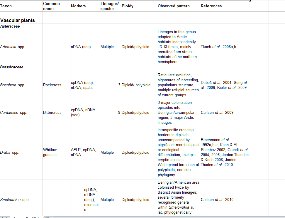
Appenidx 17.1. Selected phylogenetic studies of (or including) Arctic taxa.
-
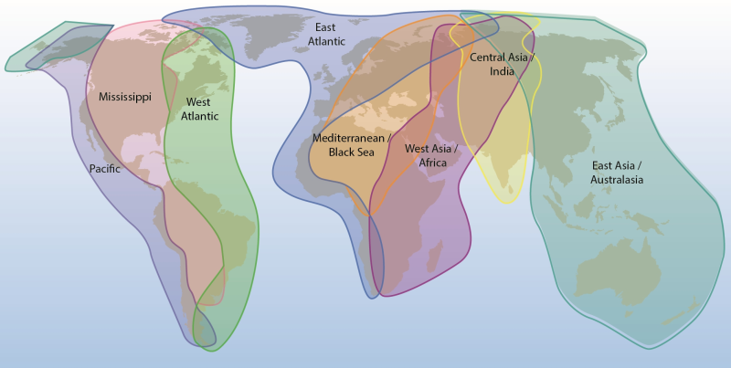
Arctic Biodiversity Assessment (ABA) 2013. Figure 4.2. Major flyways of Arctic birds. Bird migration links Arctic breeding areas to all other parts of the globe (adapted from ACIA 2005). Conservation of Arctic Flora and Fauna, CAFF 2013 - Akureyri . Arctic Biodiversity Assessment. Status and Trends in Arctic biodiversity. - Birds(Chapter 4) page 146
-
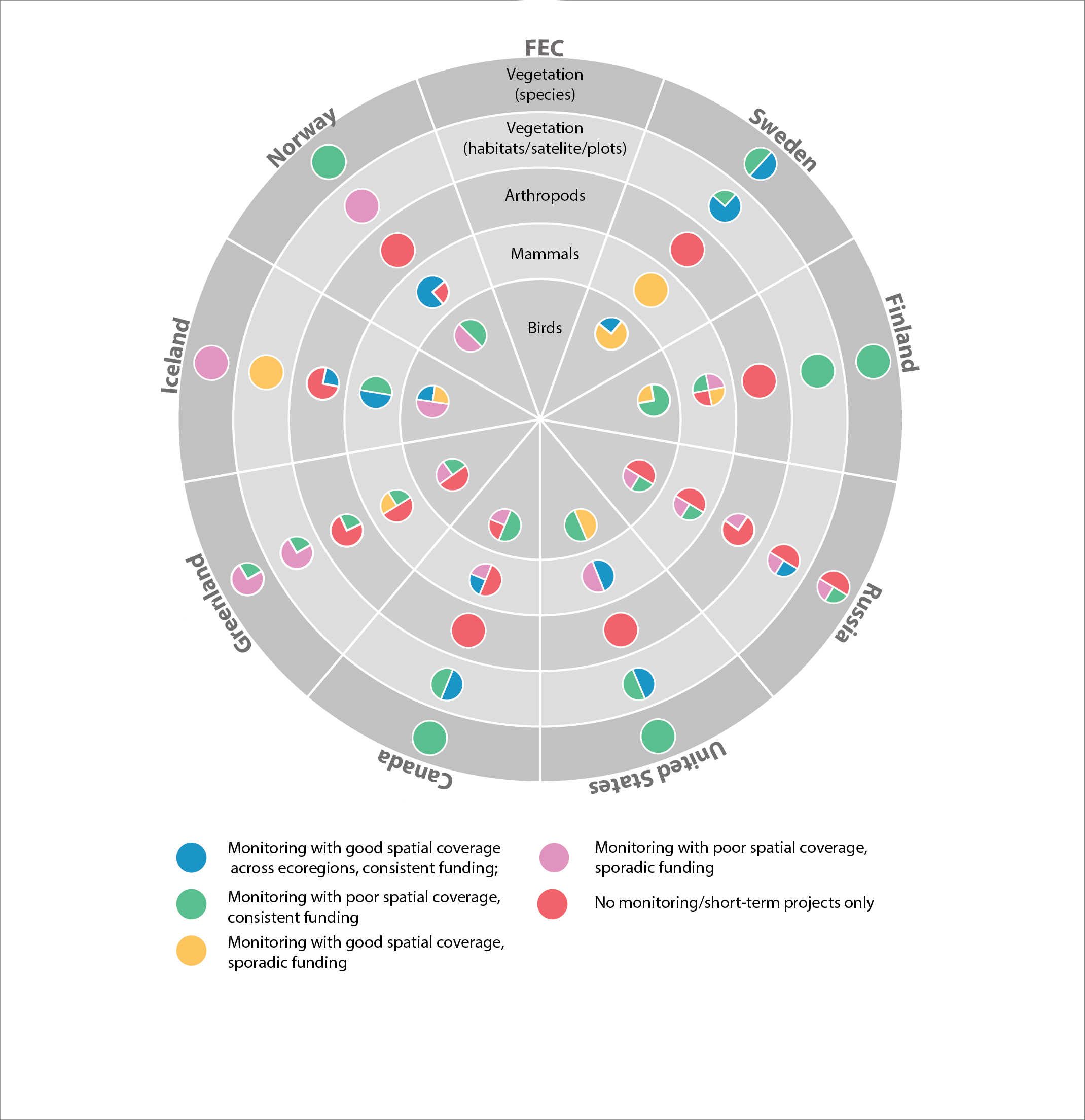
Current state of monitoring for Arctic terrestrial biodiversity FECs in each Arctic state. STATE OF THE ARCTIC TERRESTRIAL BIODIVERSITY REPORT - Chapter 4 - Page 102 - Figure 4.1
-
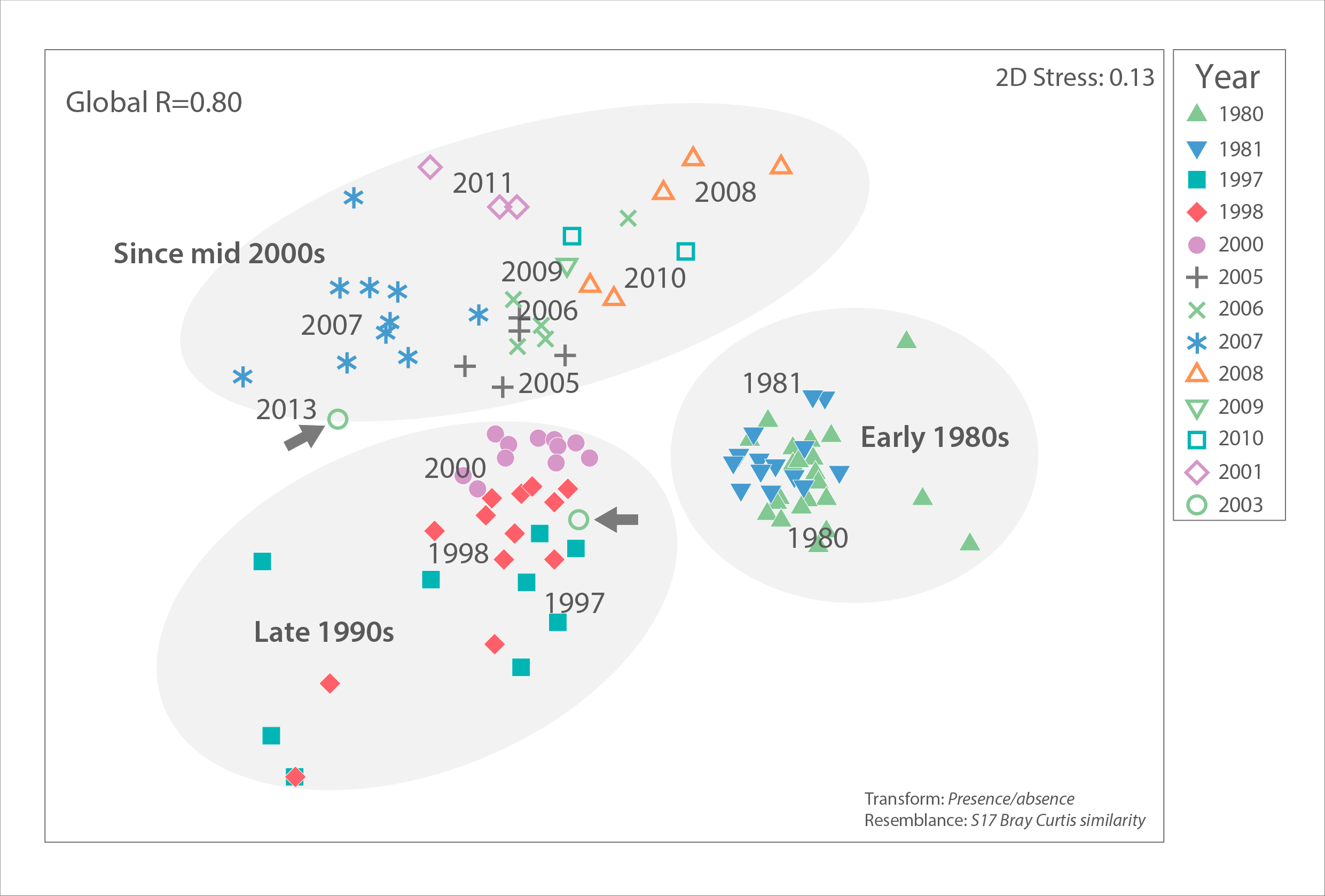
Ice algal community similarity of central Russian Arctic drifting stations from the 1980s to 2010s based on unpublished data by I.A. Melnikov, Shirshov Institute of Oceanology. The closer two samples (symbols) are to each other in this multi-dimensional scaling plot, the more similar their algal communities were, based on presence/absence of algal species. Samples from the same year tend to be similar and group together on the plot, with some exceptions. Dispersion across the plot suggests that community structure has changed over the decades, although sampling locations in the central Arctic have also shifted, thus introducing bias. An analysis of similarity (PRIMER version 6) with a high Global R=0.80 indicates strong community difference among decades (global R=0 indicates no difference, R=1 indicates complete dissimilarity). Regional differences were low (global R=0.26) and difference by ice type moderate (global R=0.38). Grey arrows point to the very different and only two samples from 2013. STATE OF THE ARCTIC MARINE BIODIVERSITY REPORT - <a href="https://arcticbiodiversity.is/findings/sea-ice-biota" target="_blank">Chapter 3</a> - Page 47 - Figure 3.1.8 "For the analysis of possible interannual trends in the ice algal community, we used a data set from the Central Arctic, the area most consistently and frequently sampled (Melnikov 2002, I. Melnikov, Shirshov Institute, unpubl. data). Multivariate community structure was analysed based on a presence-absence matrix of cores from 1980 to 2013. The analysis is biased by the varying numbers of analysed cores taken per year ranging widely from 1 to 24, ice thickness between 0.6 and 4.2 m, and including both first-year as well as multiyear sea ice. Locations included were in a bounding box within 74.9 to 90.0 °N and 179.9°W to 176.6°E and varied among years."
-
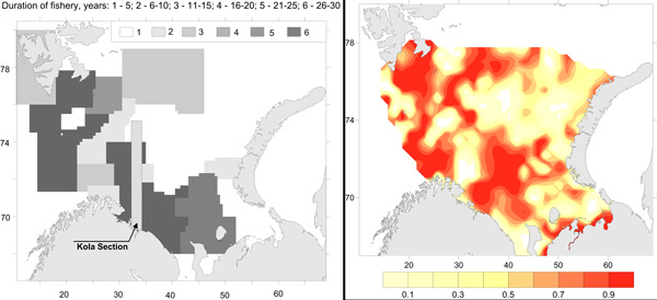
Commercial fishery impact on zoobenthos of the Barents Sea. Figure A) Intensity and duration of fishery efforts in standard commercial fishery areas in the Barents Sea. The darker the area the longer the fishery has been in operation. Figure B) Level of decline in macrobenthic biomass between 1926-1932 and 1968-1970 calculated as 1-b1968/b1930. The largest biomass decreases correspond to the darker colour, whereas lighter colour refers to no change (Denisenko 2013). STATE OF THE ARCTIC MARINE BIODIVERSITY REPORT - <a href="https://arcticbiodiversity.is/findings/benthos" target="_blank">Chapter 3</a> - Page 97 - Figure 3.3.4
-
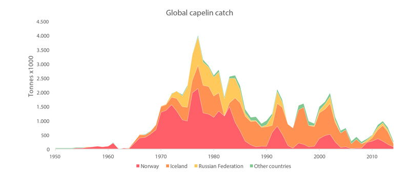
Global catches of all capelin species from 1950 to 2011 (FAO 2015). STATE OF THE ARCTIC MARINE BIODIVERSITY REPORT - <a href="https://arcticbiodiversity.is/findings/marine-fishes" target="_blank">Chapter 3</a> - Page 119 - Figure 3.4.6
-
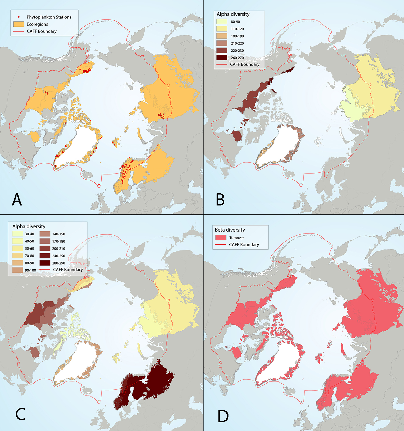
Figure 4 17 Results of circumpolar assessment of lake phytoplankton,(a) the location of phytoplankton stations, underlain by circumpolar ecoregions; (b) ecoregions with many phytoplankton stations, colored on the basis of alpha diversity rarefied to 35 stations; (c) all ecoregions with phytoplankton stations, colored on the basis of alpha diversity rarefied to 10 stations; (d) ecoregions with at least two stations in a hydrobasin, colored on the basis of the dominant component of beta diversity (species turnover, nestedness, approximately equal contribution, or no diversity) when averaged across hydrobasins in each ecoregion. State of the Arctic Freshwater Biodiversity Report - Chapter 4 - Page 56 - Figure 4-17
-
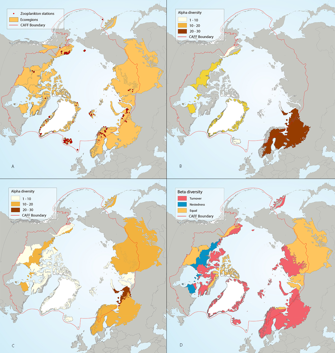
Results of circumpolar assessment of lake zooplankton, focused just on crustaceans, and indicating (a) the location of crustacean zooplankton stations, underlain by circumpolar ecoregions; (b) ecoregions with many crustacean zooplankton stations, colored on the basis of alpha diversity rarefied to 25 stations; (c) all ecoregions with crustacean zooplankton stations, colored on the basis of alpha diversity rarefied to 10 stations; (d) ecoregions with at least two stations in a hydrobasin, colored on the basis of the dominant component of beta diversity (species turnover, nestedness, approximately equal contribution, or no diversity) when averaged across hydrobasins in each ecoregion. State of the Arctic Freshwater Biodiversity Report - Chapter 4 - Page 58 - Figure 4-25
-
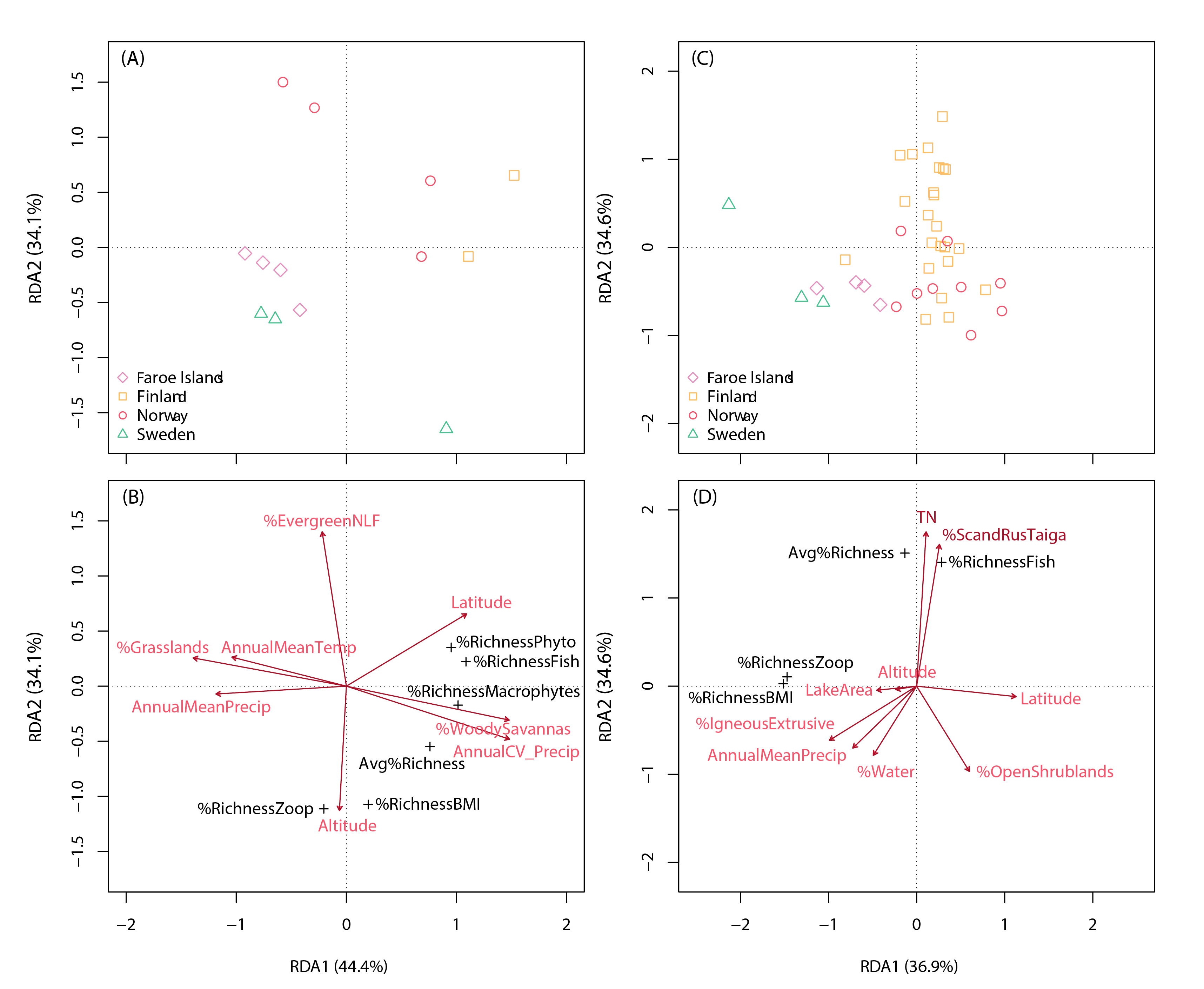
Redundancy analysis of percentage species taxa share (taxa richness relative to richness of all taxa) among 5 FECs (phytoplankton, macrophytes, zooplankton, benthic macroinvertebrates and fish) in 13 Fennoscandian lakes (panels A and B) and among 3 FECs in 39 Fennoscandian lakes (panels C and D).The upper panels show lake ordinations, while the bottom panels show explanatory environmental variables (red arrows), as indicated by permutation tests (p < 0.05). Avg%Richness: average species taxa richness as a percentage of richness of all FECs (i.e., including benthic algae if present); %Richness BMI: relative taxa share in benthic macroinvertebrates; %EvergreenNLF: percentage cover of evergreen needle-leaf forests. State of the Arctic Freshwater Biodiversity Report - Chapter 5 - Page 87 - Figure 5-4