 CAFF - Arctic Biodiversity Data Service (ABDS)
oceans
Type of resources
Available actions
Topics
Keywords
Contact for the resource
Provided by
Years
Formats
Representation types
Update frequencies
status
Scale
-
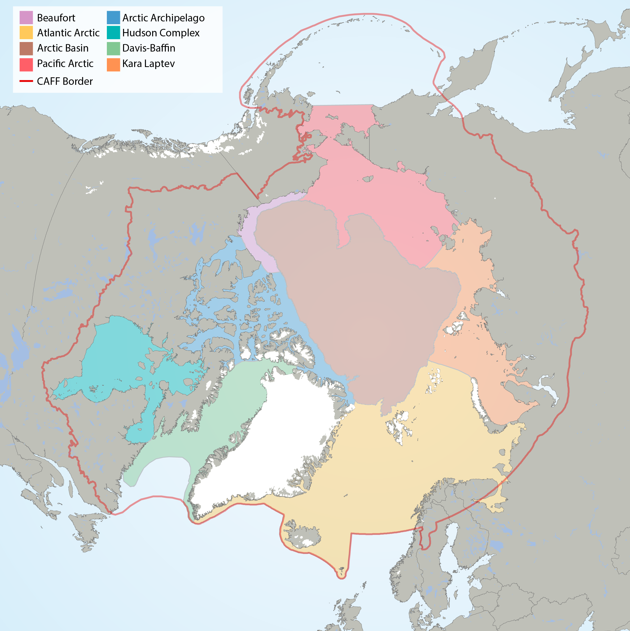
Arctic Marine Areas (AMAs) as defined in the CBMP Marine Plan. STATE OF THE ARCTIC MARINE BIODIVERSITY REPORT - <a href="https://arcticbiodiversity.is/marine" target="_blank">Chapter 1</a> - Page 15 - Figure 1.2
-
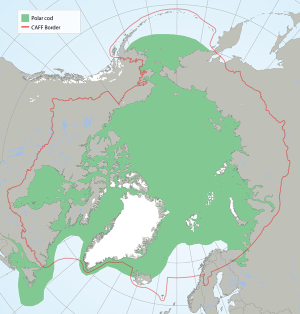
Distribution of polar cod (Boreogadus saida) based on participation in research sampling, examination of museum voucher collections and the literature (Mecklenburg et al. 2011, 2014, 2016; Mecklenburg and Steinke 2015). Map shows the maximum distribution observed from point data and includes both common and rare locations. STATE OF THE ARCTIC MARINE BIODIVERSITY REPORT - <a href="https://arcticbiodiversity.is/findings/marine-fishes" target="_blank">Chapter 3</a> - Page 114 - Figure 3.4.2
-
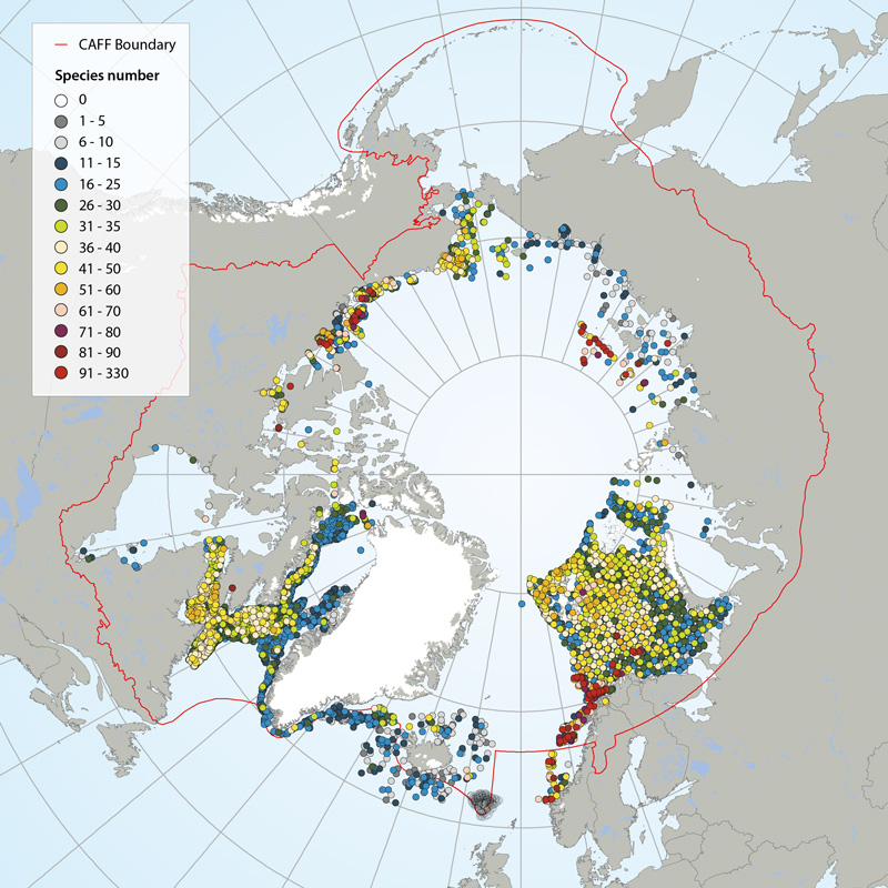
Number of megafauna species/taxa in the Arctic (7,322 stations in total), based on recent trawl investigations. Stations with highest species/taxon number are sorted to the top, meaning that dense concentrations of stations (e.g. Eastern Canada, Barents Sea), with low species numbers are hidden behind stations with higher species numbers. Also note that species numbers are somewhat biased by differing taxonomic resolution between studies. Data from: Icelandic Institute of Natural History, Iceland; Marine Research Institute, Iceland; University of Alaska, Fairbanks, U.S.; Greenland Institute of Natural Resources, Greenland; Zoological Institute of the Russian Academy of Sciences, St. Petersburg, Russia; Université du Québec à Rimouski, Canada; Fisheries and Oceans Canada; Institute of Marine Research, Norway; and Polar Research Institute of Marine Fisheries and Oceanography, Murmansk, Russia. STATE OF THE ARCTIC MARINE BIODIVERSITY REPORT - <a href="https://arcticbiodiversity.is/findings/benthos" target="_blank">Chapter 3</a> - Page 91 - Box figure 3.3.2 Several regions of the Pan Arctic have been sampled with trawl. Even though the trawl configurations and the taxonomic level are different from area to area, we choose to consider the taxonomic richness as relatively comparative.
-
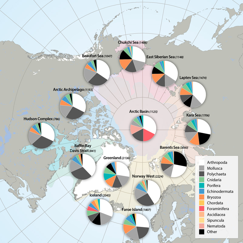
Arthropods (e.g., shrimps, crabs, sea spiders, amphipods, isopods) dominate taxon numbers in all Arctic regions, followed by polychaetes (e.g., bristle worms) and mollusks (e.g., gastropods, bivalves). Other taxon groups are diverse in some regions, such as bryozoans in the Kara Sea, cnidarians in the Atlantic Arctic, and foraminiferans in the Arctic deep-sea basins. This pattern is biased, however, by the meiofauna inclusion for the Arctic Basin (macro- and meiofauna size ranges overlap substantially in deep-sea fauna, so nematodes and foraminiferans are included) and the influence of a lack of specialists for some difficult taxonomic groups. STATE OF THE ARCTIC MARINE BIODIVERSITY REPORT - <a href="https://arcticbiodiversity.is/findings/benthos" target="_blank">Chapter 3</a> - Page 89 - Box figure 3.3.1 Each region of the Pan Arctic has been sampled with a set of different sampling gears, including grab, sledge and trawl, while other areas has only been sampled with grab. Here is the complete species/taxa number and the % distribution of species/taxa in main phyla, per region of the Pan Arctic.
-
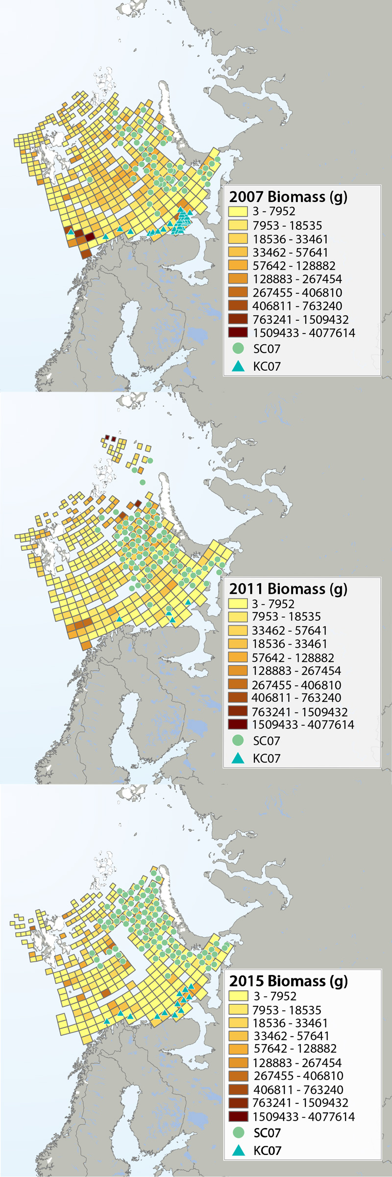
Megafauna distribution of biomass (g/15 min trawling) in the Barents Sea in 2007, 2011 and 2015. The green circles show the distribution of the snow crab as it spreads from east to west, and the blue triangles show the invasion of king crab along the coast of the southern Barents Sea. Data from Institute of Marine Research, Norway and the Polar Research Institute of Marine Fisheries and Oceanography, Murmansk, Russia. STATE OF THE ARCTIC MARINE BIODIVERSITY REPORT - <a href="https://arcticbiodiversity.is/findings/benthos" target="_blank">Chapter 3</a> - Page 95 - Figure 3.3.2 The annual joint Norwegian–Russian Ecosystem Survey provides from more than 400 stations and during extensive cruise tracks covering more or less the whole Barents Sea in August– September. The sampling is based on a regular grid spanning about 1.5 millionkm2 with fixed positions of stations which make it possible to measure changes in spatial distribution over time. The trawl is a Campelen 1800 bottom trawl rigged with rock-hopper groundgear and towed on double Warps. The mesh size is 80 mm (stretched) in the front and 16–22 mmin the cod end, allowing the capture and retention of smaller fish and the largest benthos from the seabed (benthic megafauna). The horizontal opening was 11.7 m, and the vertical opening 4–5 m (Teigsmark and Øynes, 1982). The trawl configuration and bottom contact was monitored remotely by SCANMAR trawl sensors. The standard distance between trawl stations was 35 nautical miles (65 km), except north and west of Svalbard where a stratified sampling was adapted to the steep continental shelve. The standard procedure was to tow 15 min after the trawl had made contact with the bottom, but the actual tow duration ranged between 5 min and 1 h and data were subsequently standardized to 15 min trawl time. Towing speed was 3 knots, equivalent to a towing distance of 0.75 nautical miles (1.4 km) during a 15 min tow. The trawl catches were recorded using the same procedures on the Russian and the Norwegian Research vessels to ensure comparability across Barents Sea regions. The benthic megafauna was separated from the fish and shrimp catch, washed, and sorted to lowest possible taxonomic level, in most cases to species, on-Board the vessel. Species identification was standardized between the researcher teams by annually exchanging the benthic expert’s among the vessels and taxon names were fixed each year according toWORMSwhen possible.This resulted in an Electronic identification manual and photo-compendium as a tool to standardize taxon identifications, in addition to various sources of identification literature. Difficult taxa were photographed and, in some cases, brought back as preserved voucher specimens for further identification. Wet-weight biomass was recorded with electronic scales in the ship laboratories for each taxon.The biomass determination included all fragments.
-
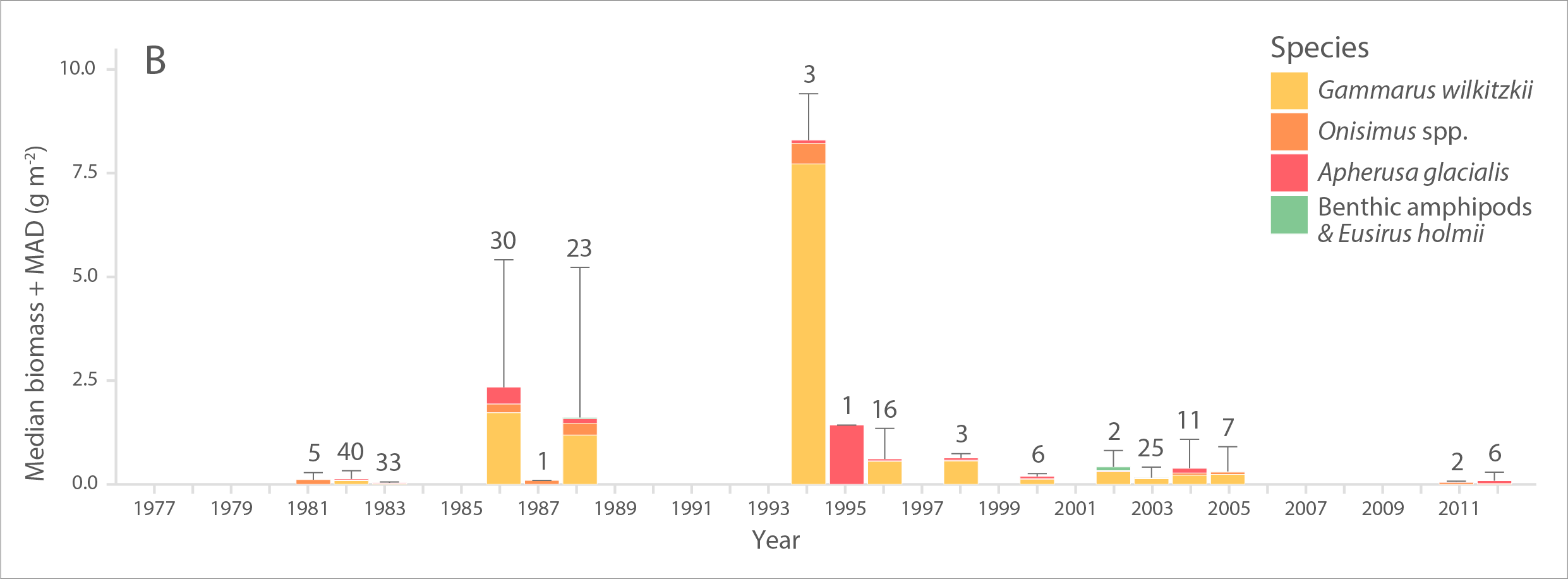
Multi-decadal time series of A) abundance (individuals m-2) and B) biomass (g wet weight m-2) of ice amphipods from 1977 to 2012 across the Arctic. Bars and error bars indicate median and median absolute deviation (MAD) values for each year, respectively. Numbers above bars represent number of sampling efforts (n). Modified from Hop et al. (2013). STATE OF THE ARCTIC MARINE BIODIVERSITY REPORT - <a href="https://arcticbiodiversity.is/findings/sea-ice-biota" target="_blank">Chapter 3</a> - Page 45 - Figure 3.1.7 From the report draft: "The only available time-series of sympagic biota is based on composite data of ice-amphipod abundance and biomass estimates from the 1980s to present across the Arctic, with most observations from the Svalbard and Fram Strait region (Hop et al. 2013). Samples were obtained by SCUBA divers who collected amphipods quantitatively with electrical suction pumps under the sea ice (Lønne & Gulliksen 1991a, b, Hop & Pavlova 2008)."
-
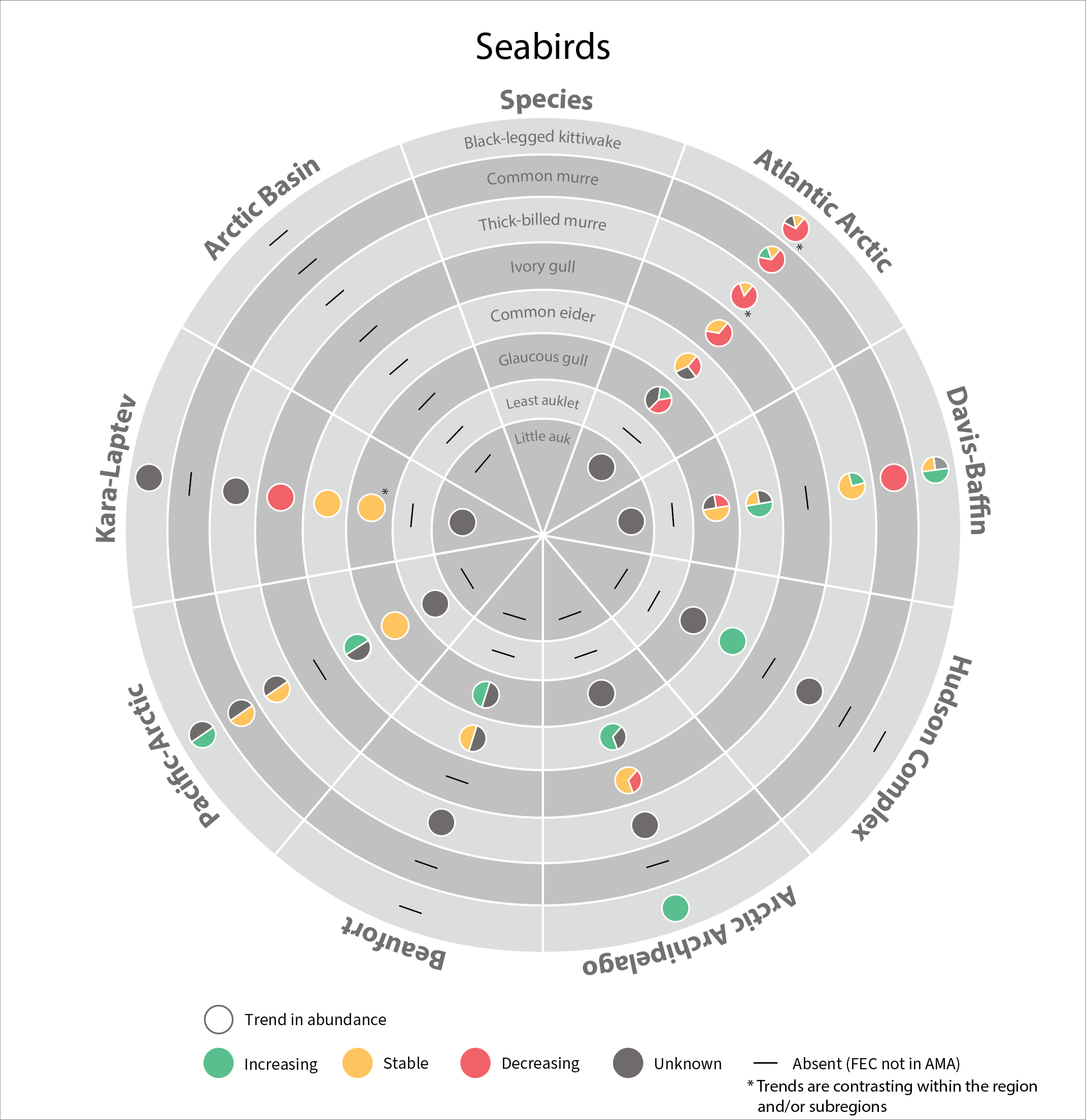
In 2017, the SAMBR synthesized data about biodiversity in Arctic marine ecosystems around the circumpolar Arctic. SAMBR highlighted observed changes and relevant monitoring gaps using data compiled through 2015. In 2021 an update was provided on the status of seabirds in circumpolar Arctic using data from 2016–2019. Most changes reflect access to improved population estimates, orimproved data for monitoring trends,independent of recognized trends in population size.
-
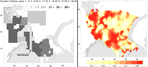
Commercial fishery impact on zoobenthos of the Barents Sea. Figure A) Intensity and duration of fishery efforts in standard commercial fishery areas in the Barents Sea. The darker the area the longer the fishery has been in operation. Figure B) Level of decline in macrobenthic biomass between 1926-1932 and 1968-1970 calculated as 1-b1968/b1930. The largest biomass decreases correspond to the darker colour, whereas lighter colour refers to no change (Denisenko 2013). STATE OF THE ARCTIC MARINE BIODIVERSITY REPORT - <a href="https://arcticbiodiversity.is/findings/benthos" target="_blank">Chapter 3</a> - Page 97 - Figure 3.3.4
-
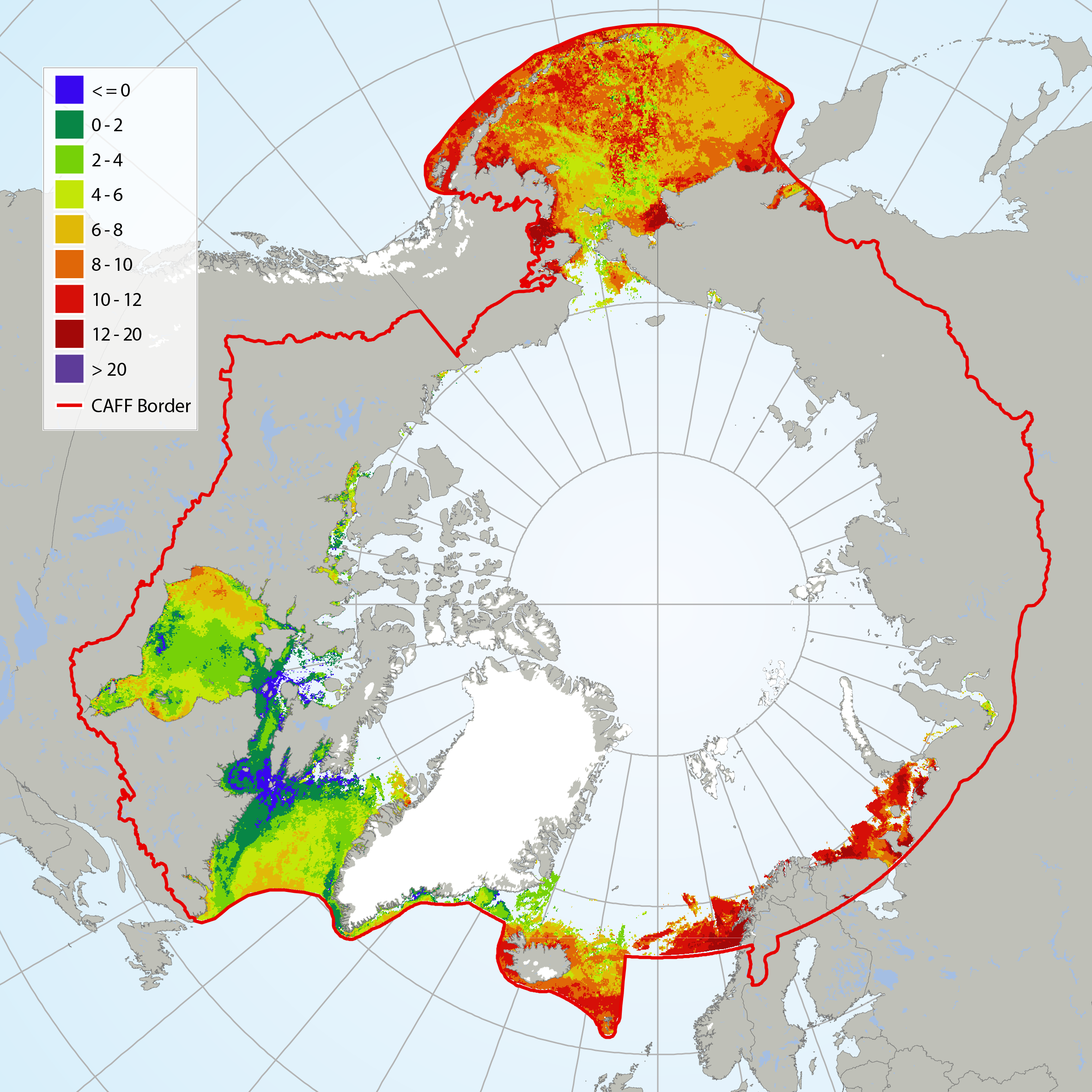
It has not been possible to identify available trend data for Arctic Ocean sea surface temperatures because there is not enough data to calculate reliable long-term trends for much of the Arctic marine environment (IPCC 2013, NOAA 2015). Here, sea surface temperature for July 2015 is shown from CAFF’s Land Cover Change Index. MODIS Sea Surface Temperature (SST) provided a four-kilometre spatial resolution monthly composite snapshot made from night-time measurements from the NASA Aqua Satellite. The night-time measurements are used to collect a consistent temperature measurement that is unaffected by the warming of the top layer of water by the sun. STATE OF THE ARCTIC MARINE BIODIVERSITY REPORT - <a href="https://arcticbiodiversity.is/marine" target="_blank">Chapter 2</a> - Page 25 - Figure 2.3
-
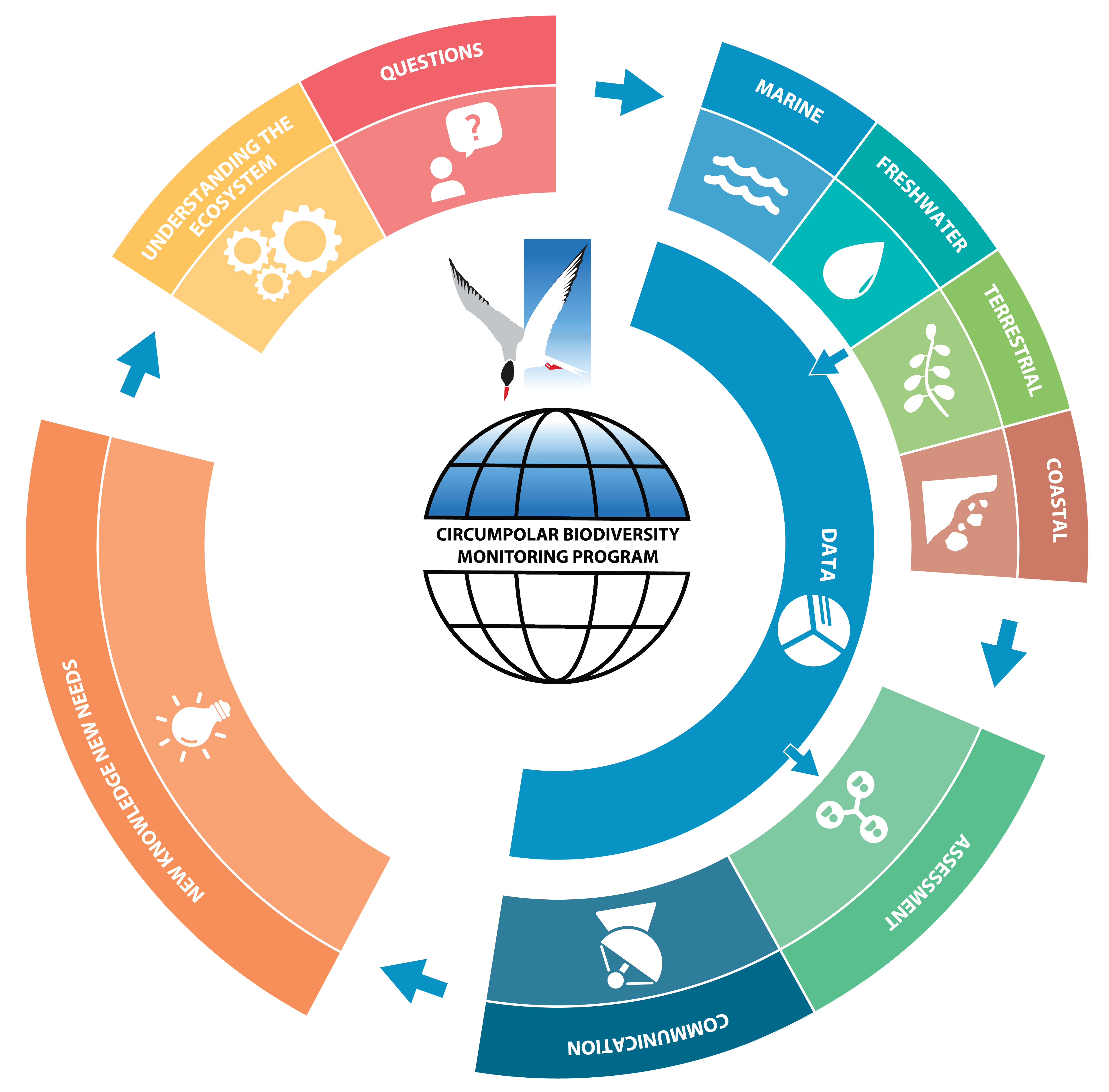
Workflow of the Circumpolar Biodiversity Monitoring Program (CBMP). STATE OF THE ARCTIC MARINE BIODIVERSITY REPORT - <a href="https://arcticbiodiversity.is/marine" target="_blank">Chapter 1</a> - Page 13 - Figure 1.1