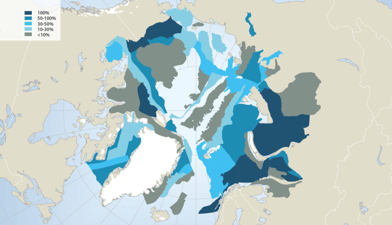
Extensive oil and gas activity has occurred in the Arctic, primarily land-based, with Russia extracting 80% of the oil and 99% of the gas to date (AMAP 2008). Furthermore, the Arctic still contains large petroleum hydrocarbon reserves and potentially holds one fifth of the world’s yet undiscovered resources, according to the US Geological Survey (USGS 2008) (Fig. 14.4). While much of the currently known Arctic oil and gas reserves are in Russia (75% of oil and 90% of gas; AMAP 2008), more than half of the estimated undiscovered Arctic oil reserves are in Alaska (offshore and onshore), the Amerasian Basin (offshore north of the Beaufort Sea) and in W and E Greenland (offshore). More than 70% of the Arctic undiscovered natural gas is estimated to be located in the W Siberian Basin (Yamal Peninsula and offshore in the Kara Sea), the E Barents Basin and in Alaska (offshore and onshore) (AMSA 2009). Associated with future exploration and development, each of these regions would require vastly expanded Arctic marine operations, and several regions such as offshore Greenland would require fully developed Arctic marine transport systems to carry hydrocarbons to global markets. In this context, regions of high interest for economic development face cumulative environmental pressure from anthropogenic activities such as hydrocarbon exploitation locally, together with global changes associated with climatic and oceanographic trends. Conservation of Arctic Flora and Fauna, CAFF 2013 - Akureyri . Arctic Biodiversity Assessment. Status and Trends in Arctic biodiversity. - Marine ecosystems (Chapter 14 - page 501). Figure adapted from the USGS

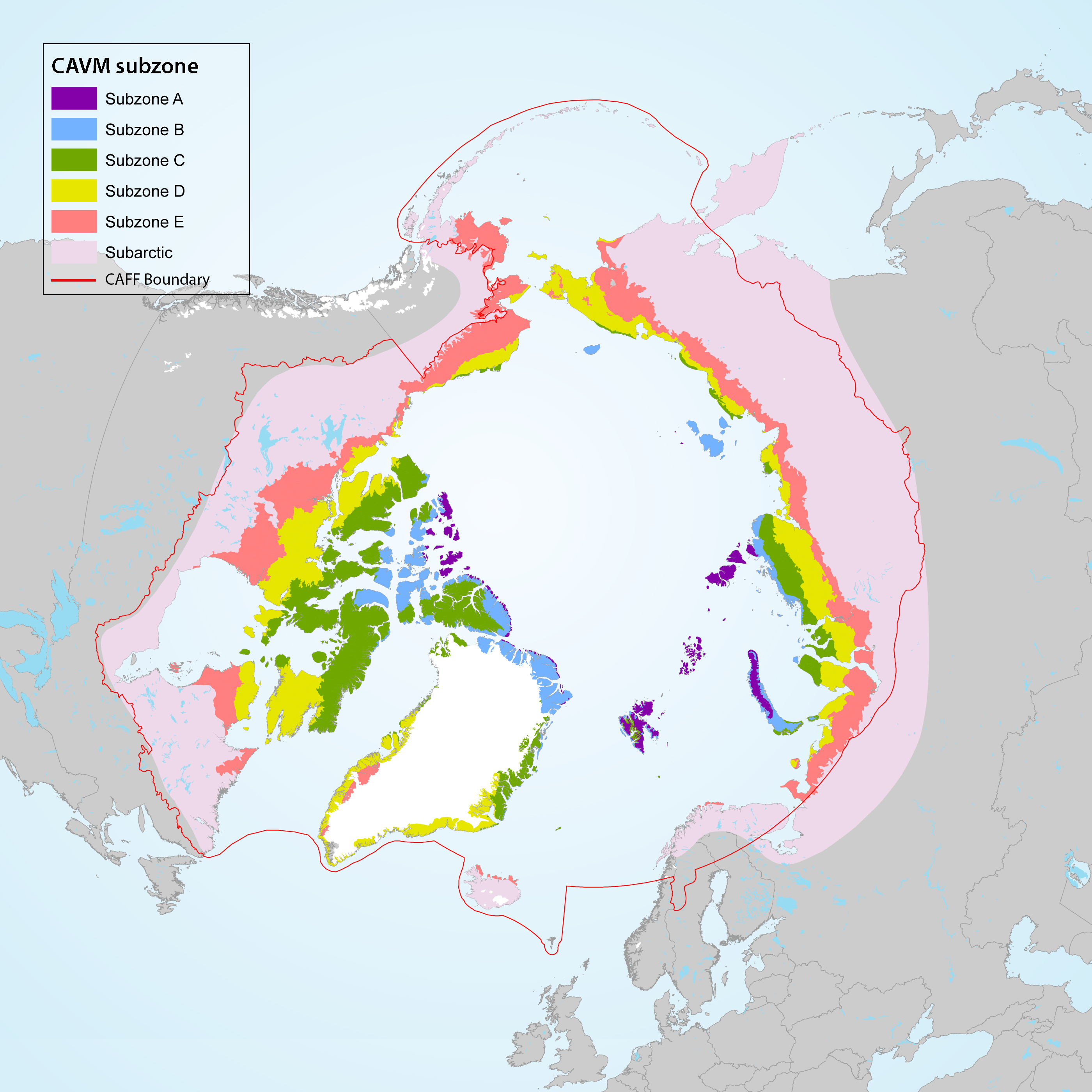
Geographic area covered by the Arctic Biodiversity Assessment and the CBMP–Terrestrial Plan. Subzones A to E are depicted as defined in the Circumpolar Arctic Vegetation Map (CAVM Team 2003). Subzones A, B and C are the high Arctic while subzones D and E are the low Arctic. Definition of high Arctic, low Arctic, and sub-Arctic follow Hohn & Jaakkola 2010. STATE OF THE ARCTIC TERRESTRIAL BIODIVERSITY REPORT - Chapter 1 - Page 14 - Figure 1.2

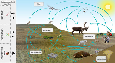
The Arctic terrestrial food web includes the exchange of energy and nutrients. Arrows to and from the driver boxes indicate the relative effect and counter effect of different types of drivers on the ecosystem. STATE OF THE ARCTIC TERRESTRIAL BIODIVERSITY REPORT - Chapter 2 - Page 26- Figure 2.4

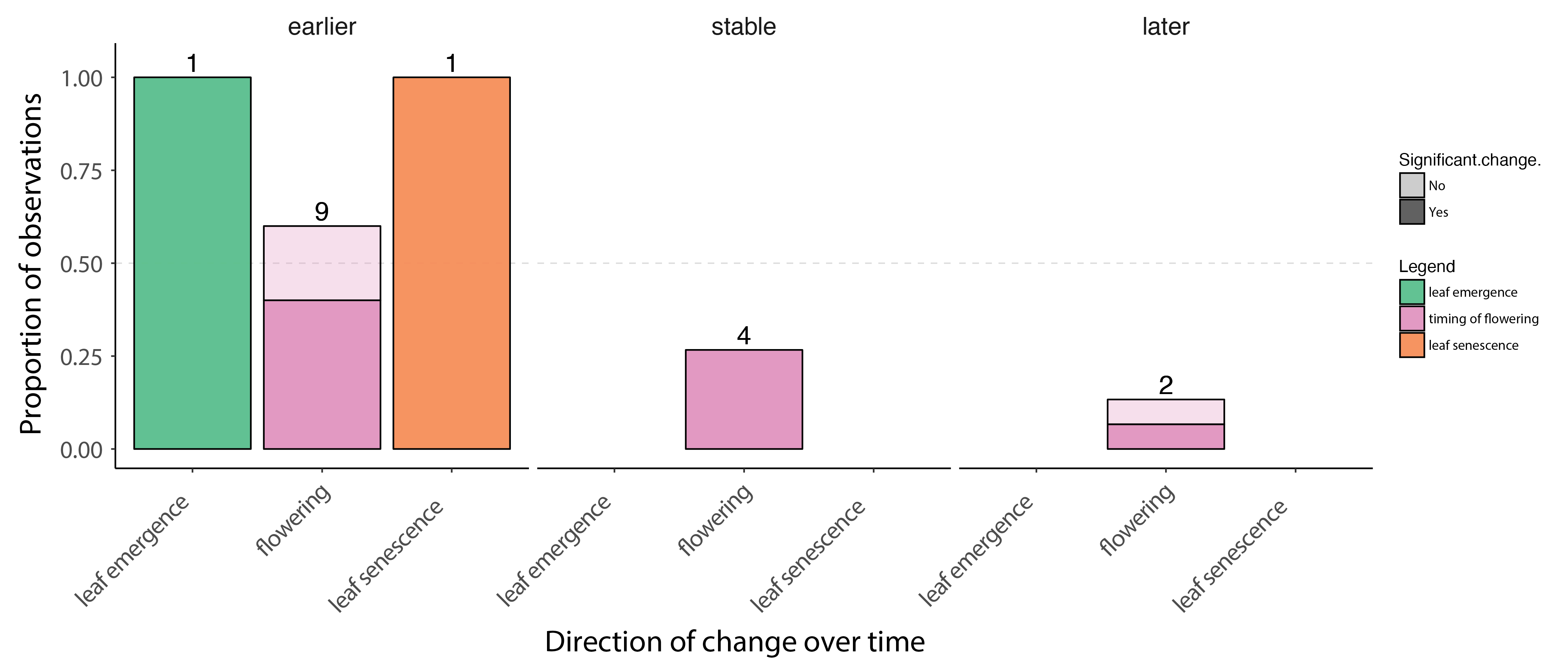
Change in plant phenology over time based on published studies, ranging from 9 to 21 years of duration. The bars show the proportion of observations where timing of phenological events advanced (earlier) was stable or were delayed (later) over time. The darker portions of each bar represent visible decrease, stable state, or increase results, and lighter portions represent marginally significant change. The numbers above each bar indicate the number of observations in that group. Figure from Bjorkman et al. 2020. STATE OF THE ARCTIC TERRESTRIAL BIODIVERSITY REPORT - Chapter 3 - Page 31- Figure 3.3

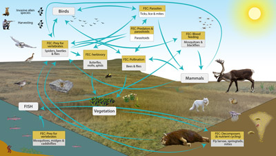
Conceptual model of the FECs and processes mediated by more than 2,500 species of Arctic arthropods known from Greenland, Iceland, Svalbard, and Jan Mayen. STATE OF THE ARCTIC TERRESTRIAL BIODIVERSITY REPORT - Chapter 3 - Page 37- Figure 3.7

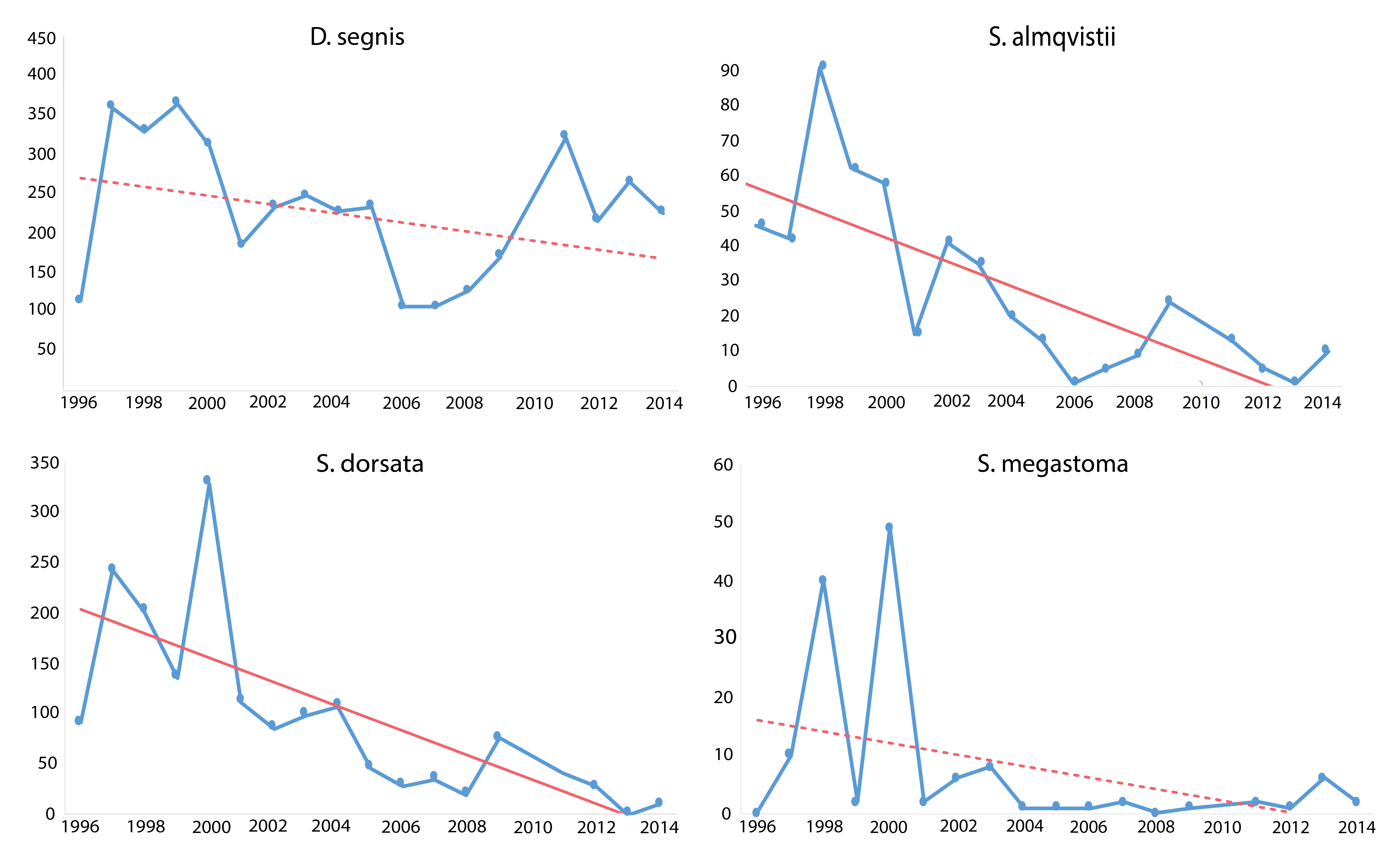
Trends in four muscid species occurring at Zackenberg Research Station, east Greenland, 1996–2014. Declines were detected in several species over five or more years. Significant regression lines drawn as solid. Non-significant as dotted lines. Modified from Gillespie et al. 2020a. (in the original figure six species showed a statistically significant decline, seven a non-significant decline and one species a non-significant rise) STATE OF THE ARCTIC TERRESTRIAL BIODIVERSITY REPORT - Chapter 3 - Page 39 - Figure 3.11

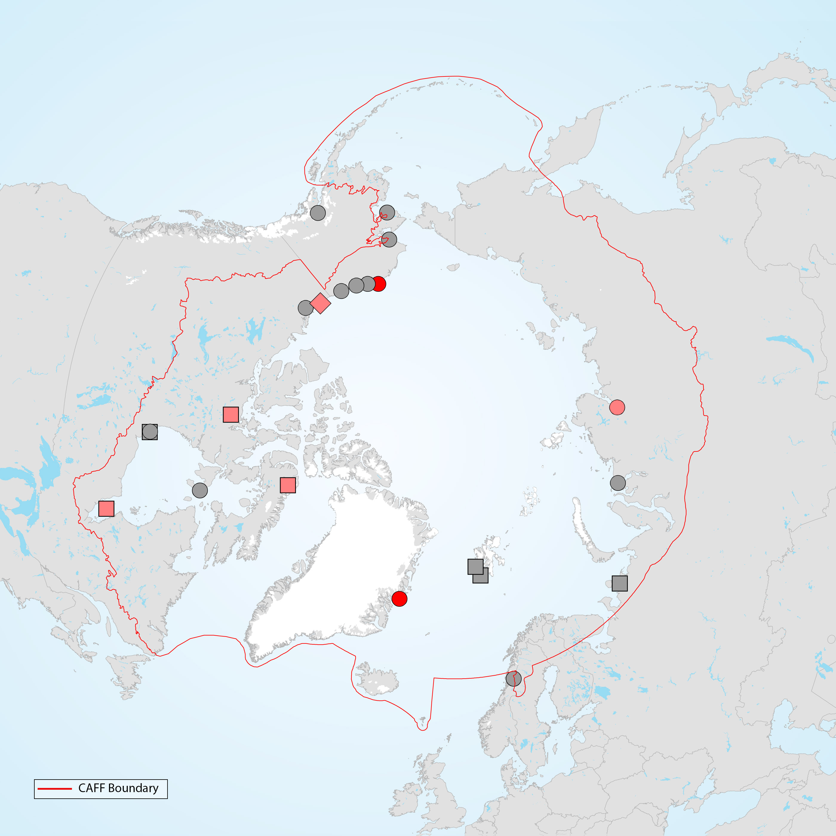
Study sites across the Arctic where phenological mismatches between timing of reproduction and peak abundance in food have been studied for terrestrial bird species. Grey symbols show study sites where this phenomenon has been studied for <10 years, light red symbols show sites with >10 years of data but no strong evidence of an increasing mismatch, and dark red symbols indicate sites with >10 years of data and strong evidence of an increasing mismatch. Circles indicate studies of shorebirds, squares for waterfowl and diamonds(triancle) for both shorebirds and passerines. Graphic: Thomas Lameris, adapted from Zhemchuzhnikov (submitted). STATE OF THE ARCTIC TERRESTRIAL BIODIVERSITY REPORT - Chapter 3 - Page 65 - Figure Box 3.3

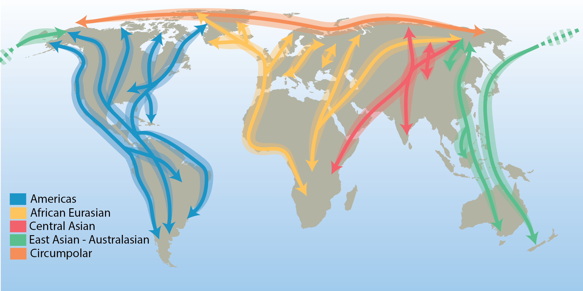
There are few true Arctic specialist birds that remain in the Arctic throughout their annual cycle. They include the willow and rock ptarmigan (Lagopus lagopus and L. muta), gyrfalcon (Falco rusticolus), snowy owl (Bubo scandiacus), Arctic redpoll (Carduelis hornemanni) and northern raven (Corvus corax)—a cosmopolitan species with resident populations in the Arctic. All other terrestrial Arctic-breeding bird species migrate to warmer regions during the northern winter, connecting the Arctic to all corners of the globe. Hence, their distributions are influenced by the routes they follow. These distinct migration routes are referred to as flyways and are defined by a combination of ecological and political boundaries and differ in spatial scale. The CBMP refers to the traditional four north–south flyways, in addition to a circumpolar flyway representing the few species that remain largely within the Arctic year-round (Figure 3-20). STATE OF THE ARCTIC TERRESTRIAL BIODIVERSITY REPORT - Chapter 3 - Page 48- Figure 3.20

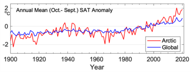
Warming in the Arctic has been significantly faster than anywhere else on Earth (Ballinger et al. 2020). Trends in land surface temperature are shown on Figure 2-2. STATE OF THE ARCTIC TERRESTRIAL BIODIVERSITY REPORT - Chapter 2 - Page 23 - Figure 2.2

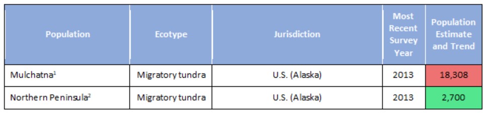
Population estimates and trends for Rangifer populations of the migratory tundra, Arctic island, mountain, and forest ecotypes where their circumpolar distribution intersects the CAFF boundary. Population trends (Increasing, Stable, Decreasing, or Unknown) are indicated by shading. Data sources for each population are indicated as footnotes. STATE OF THE ARCTIC TERRESTRIAL BIODIVERSITY REPORT - Chapter 3 - Page 70 - Table 3.4