 CAFF - Arctic Biodiversity Data Service (ABDS)
marine
Type of resources
Available actions
Topics
Keywords
Contact for the resource
Provided by
Years
Formats
Representation types
Update frequencies
status
Scale
-
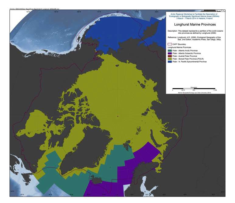
This dataset represents a partition of the world oceans into provinces as defined by Longhurst (1995; 1998; 2006), and are based on the prevailing role of physical forcing as a regulator of phytoplankton distribution. The dataset represents the initial static boundaries developed at the Bedford Institute of Oceanography, Canada. Note that the boundaries of these provinces are not fixed in time and space, but are dynamic and move under seasonal and interannual changes in physical forcing. At the first level of reduction, Longhurst recognized four principal biomes (also referred to as domains in earlier publications): the Polar Biome, the Westerlies Biome, the Trade-Winds Biome, and the Coastal Boundary Zone Biome. These four Biomes are recognizable in every major ocean basin. At the next level of reduction, the ocean basins are partitioned into provinces, roughly ten for each basin. These partitions provide a template for data analysis or for making parameter assignments on a global scale. (source: VLIZ (2009). Longhurst Biogeographical Provinces. Available online at <a href="http://www.marineregions.org/" target="_blank">Longhurst Biogeographical Provinces</a> References: Longhurst, A.R. (2006). Ecological Geography of the Sea. 2nd Edition. Academic Press, San Diego, 560p. Data available from: <a href="http://www.marineregions.org/sources.php#longhurst" target="_blank">Ecological Geography of the Sea</a>
-

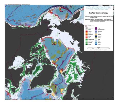
We present the first digital seafloor geomorphic features map (GSFM) of the global ocean. The GSFM includes 131,192 separate polygons in 29 geomorphic feature categories, used here to assess differences between passive and active continental margins as well as between 8 major ocean regions (the Arctic, Indian, North Atlantic, North Pacific, South Atlantic, South Pacific and the Southern Oceans and the Mediterranean and Black Seas). The GSFM provides quantitative assessments of differences between passive and active margins: continental shelf width of passive margins (88 km) is nearly three times that of active margins (31 km); the average width of active slopes (36 km) is less than the average width of passive margin slopes (46 km); active margin slopes contain an area of 3.4 million km2 where the gradient exceeds 5°, compared with 1.3 million km2 on passive margin slopes; the continental rise covers 27 million km2 adjacent to passive margins and less than 2.3 million km2 adjacent to active margins. Examples of specific applications of the GSFM are presented to show that: 1) larger rift valley segments are generally associated with slow-spreading rates and smaller rift valley segments are associated with fast spreading; 2) polar submarine canyons are twice the average size of non-polar canyons and abyssal polar regions exhibit lower seafloor roughness than non-polar regions, expressed as spatially extensive fan, rise and abyssal plain sediment deposits – all of which are attributed here to the effects of continental glaciations; and 3) recognition of seamounts as a separate category of feature from ridges results in a lower estimate of seamount number compared with estimates of previous workers. Reference: Harris PT, Macmillan-Lawler M, Rupp J, Baker EK Geomorphology of the oceans. Marine Geology.
-
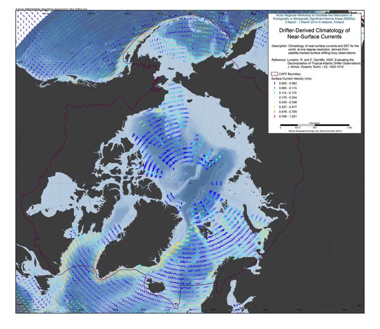
Satellite-tracked SVP drifting buoys (Sybrandy and Niiler, 1991; Niiler, 2001) provide observations of near-surface circulation at unprecedented resolution. In September 2005, the Global Drifter Array became the first fully realized component of the Global Ocean Observing System when it reached an array size of 1250 drifters. A drifter is composed of a surface float which includes a transmitter to relay data, a thermometer which reads temperature a few centimeters below the air/sea interface, and a submergence sensor used to detect when/if the drogue is lost. The surface float is tethered to a subsurface float which minimizes rectification of surface wave motion (Niiler et al., 1987; Niiler et al., 1995). This in turn is tethered to a holey sock drogue, centered at 15 m depth. The drifter follows the flow integrated over the drogue depth, although some slip with respect to this motion is associated with direct wind forcing (Niiler and Paduan, 1995). This slip is greatly enhanced in drifters which have lost their drogues (Pazan and Niiler, 2000). Drifter velocities are derived from finite differencing their raw position fixes. These velocities, and the concurrent SST measurements, are archived at <a href="http://www.aoml.noaa.gov/phod/dac/dacdata.php" target="_blank">AOML's Drifting Buoy Data Assembly Center</a> where the data are quality controlled and interpolated to 1/4-day intervals (Hansen and Herman, 1989; Hansen and Poulain, 1996). Reference: Lumpkin, R. and Z. Garraffo, 2005: Evaluating the Decomposition of Tropical Atlantic Drifter Observations. J. Atmos. Oceanic Techn. I 22, 1403-1415.
-

We present the first digital seafloor geomorphic features map (GSFM) of the global ocean. The GSFM includes 131,192 separate polygons in 29 geomorphic feature categories, used here to assess differences between passive and active continental margins as well as between 8 major ocean regions (the Arctic, Indian, North Atlantic, North Pacific, South Atlantic, South Pacific and the Southern Oceans and the Mediterranean and Black Seas). The GSFM provides quantitative assessments of differences between passive and active margins: continental shelf width of passive margins (88 km) is nearly three times that of active margins (31 km); the average width of active slopes (36 km) is less than the average width of passive margin slopes (46 km); active margin slopes contain an area of 3.4 million km2 where the gradient exceeds 5°, compared with 1.3 million km2 on passive margin slopes; the continental rise covers 27 million km2 adjacent to passive margins and less than 2.3 million km2 adjacent to active margins. Examples of specific applications of the GSFM are presented to show that: 1) larger rift valley segments are generally associated with slow-spreading rates and smaller rift valley segments are associated with fast spreading; 2) polar submarine canyons are twice the average size of non-polar canyons and abyssal polar regions exhibit lower seafloor roughness than non-polar regions, expressed as spatially extensive fan, rise and abyssal plain sediment deposits – all of which are attributed here to the effects of continental glaciations; and 3) recognition of seamounts as a separate category of feature from ridges results in a lower estimate of seamount number compared with estimates of previous workers. Reference: Harris PT, Macmillan-Lawler M, Rupp J, Baker EK Geomorphology of the oceans. Marine Geology.
-
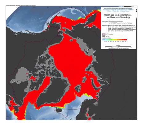
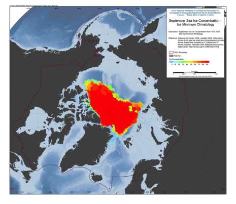
The U.S. National Ice Center (NIC) is an inter-agency sea ice analysis and forecasting center comprised of the Department of Commerce/NOAA, the Department of Defense/U.S. Navy, and the Department of Homeland Security/U.S. Coast Guard components. Since 1972, NIC has produced Arctic and Antarctic sea ice charts. This data set is comprised of Arctic sea ice concentration climatology derived from the NIC weekly or biweekly operational ice-chart time series. The charts used in the climatology are from 1972 through 2007; and the monthly climatology products are median, maximum, minimum, first quartile, and third quartile concentrations, as well as frequency of occurrence of ice at any concentration for the entire period of record as well as for 10-year and 5-year periods. NIC charts are produced through the analyses of available in situ, remote sensing, and model data sources. They are generated primarily for mission planning and safety of navigation. NIC charts generally show more ice than do passive microwave derived sea ice concentrations, particularly in the summer when passive microwave algorithms tend to underestimate ice concentration. The record of sea ice concentration from the NIC series is believed to be more accurate than that from passive microwave sensors, especially from the mid-1990s on (see references at the end of this documentation), but it lacks the consistency of some passive microwave time series. Source: <a href="http://nsidc.org/data/G02172" target="_blank">NSIDC</a> Reference: National Ice Center. 2006, updated 2009. National Ice Center Arctic sea ice charts and climatologies in gridded format. Edited and compiled by F. Fetterer and C. Fowler. Boulder, Colorado USA: National Snow and Ice Data Center. Source: <a href="http://nsidc.org/data/G02172" target="_blank">NSIDC</a>
-
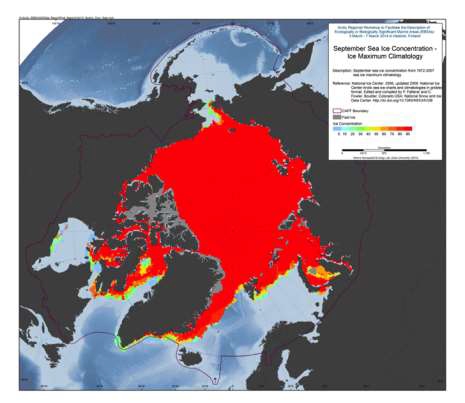
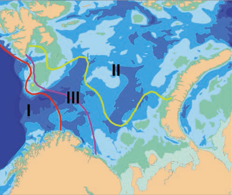
Biogeographic borders in the Barents Sea based on species distributions of bryozoans. Average position of the border with 50:50% of Atlantic boreal and Arctic species numbers is indicated by the pink line, and the red and green lines indicate the extreme positions of the border in cold and warm periods respectively. Area III between them is the transitional zone between the Atlantic boreal and the Arctic regions. Thus, area I always has > 50% Atlantic boreal species, and area II always > 50% Arctic species (after Denisenko 1990).
-
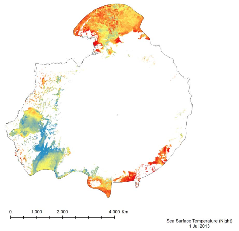
The MODIS Sea Surface Temperature (SST) product provided is a 4km spatialresolution monthly composite made from nighttime measurements from the Aqua Satellite.The nighttime measurements are used to collect a consistent temperature measurement that isunaffected by the warming of the top layer of water by the sun.