 CAFF - Arctic Biodiversity Data Service (ABDS)
Land use
Type of resources
Available actions
Topics
Keywords
Contact for the resource
Provided by
Years
Representation types
Update frequencies
status
-
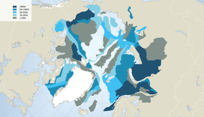
Extensive oil and gas activity has occurred in the Arctic, primarily land-based, with Russia extracting 80% of the oil and 99% of the gas to date (AMAP 2008). Furthermore, the Arctic still contains large petroleum hydrocarbon reserves and potentially holds one fifth of the world’s yet undiscovered resources, according to the US Geological Survey (USGS 2008) (Fig. 14.4). While much of the currently known Arctic oil and gas reserves are in Russia (75% of oil and 90% of gas; AMAP 2008), more than half of the estimated undiscovered Arctic oil reserves are in Alaska (offshore and onshore), the Amerasian Basin (offshore north of the Beaufort Sea) and in W and E Greenland (offshore). More than 70% of the Arctic undiscovered natural gas is estimated to be located in the W Siberian Basin (Yamal Peninsula and offshore in the Kara Sea), the E Barents Basin and in Alaska (offshore and onshore) (AMSA 2009). Associated with future exploration and development, each of these regions would require vastly expanded Arctic marine operations, and several regions such as offshore Greenland would require fully developed Arctic marine transport systems to carry hydrocarbons to global markets. In this context, regions of high interest for economic development face cumulative environmental pressure from anthropogenic activities such as hydrocarbon exploitation locally, together with global changes associated with climatic and oceanographic trends. Conservation of Arctic Flora and Fauna, CAFF 2013 - Akureyri . Arctic Biodiversity Assessment. Status and Trends in Arctic biodiversity. - Marine ecosystems (Chapter 14 - page 501). Figure adapted from the USGS
-
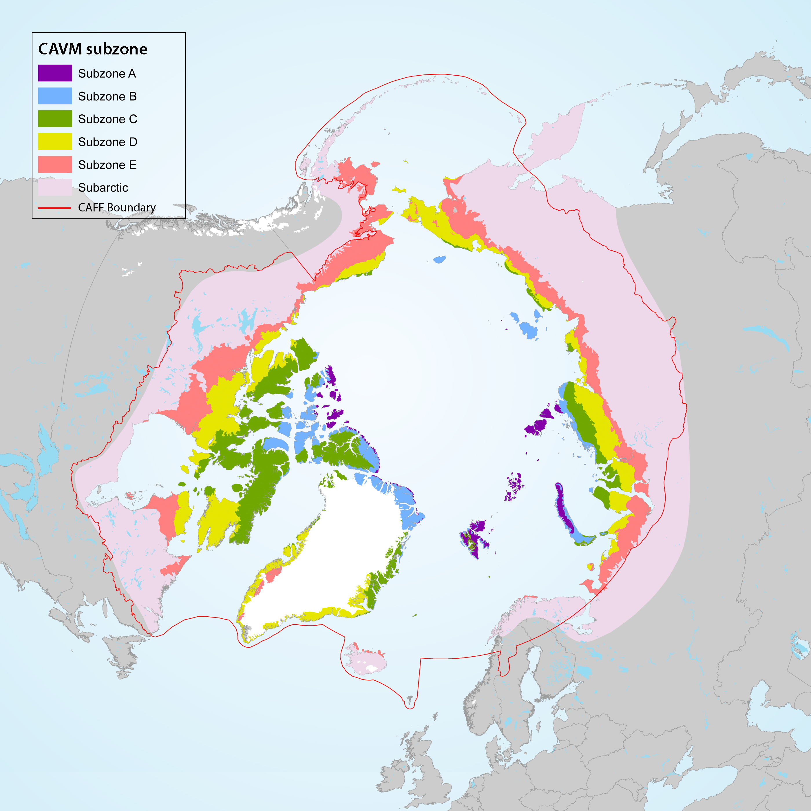
Geographic area covered by the Arctic Biodiversity Assessment and the CBMP–Terrestrial Plan. Subzones A to E are depicted as defined in the Circumpolar Arctic Vegetation Map (CAVM Team 2003). Subzones A, B and C are the high Arctic while subzones D and E are the low Arctic. Definition of high Arctic, low Arctic, and sub-Arctic follow Hohn & Jaakkola 2010. STATE OF THE ARCTIC TERRESTRIAL BIODIVERSITY REPORT - Chapter 1 - Page 14 - Figure 1.2
-
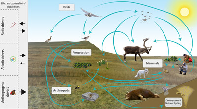
The Arctic terrestrial food web includes the exchange of energy and nutrients. Arrows to and from the driver boxes indicate the relative effect and counter effect of different types of drivers on the ecosystem. STATE OF THE ARCTIC TERRESTRIAL BIODIVERSITY REPORT - Chapter 2 - Page 26- Figure 2.4
-
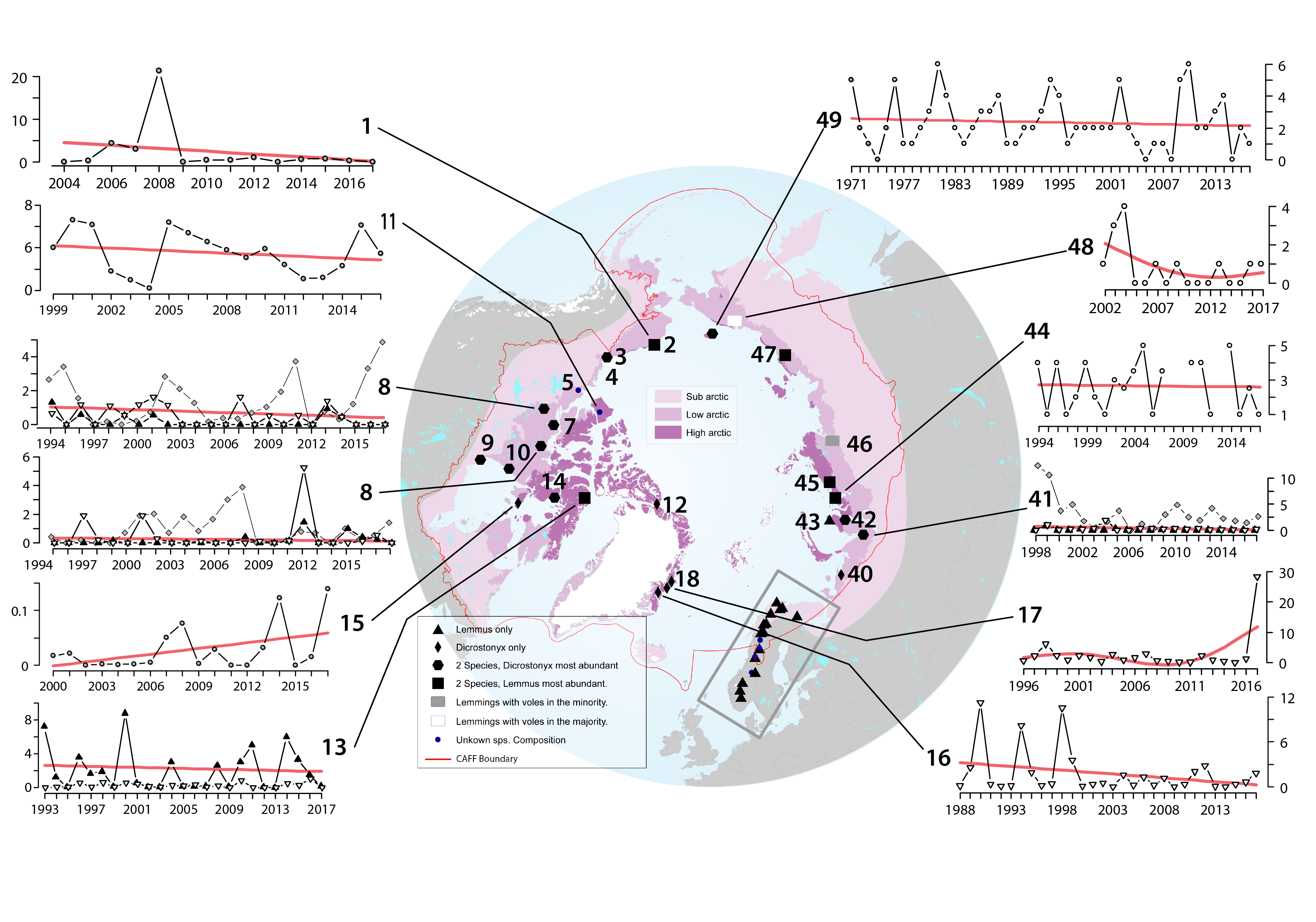
Lemmings are currently being monitored at 38 sites. Their status and trends were determined based on data from these sites as well as recent data (since 2000) from an additional 11 previous monitoring sites (Figure 3-31). Of those sites monitored, Fennoscandia is overrepresented relative to the geographical area it covers, whereas Russia is underrepresented. Based on the skewed geographical coverage, more information is available for some species of lemmings than others, particularly the Norwegian lemming. STATE OF THE ARCTIC TERRESTRIAL BIODIVERSITY REPORT - Chapter 3 - Page 80 - Figure 3.31
-
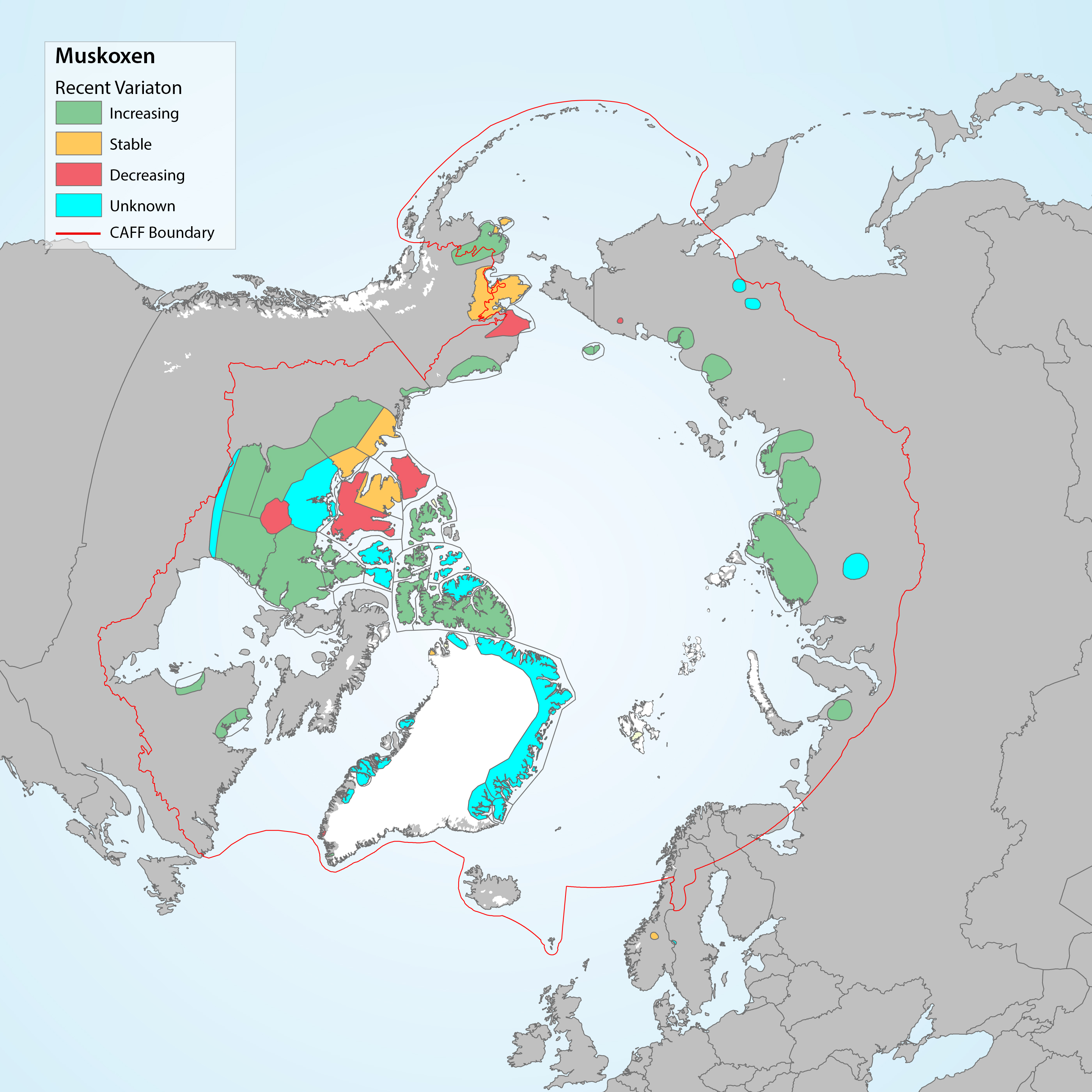
Trends and distribution of muskoxen populations based on Table 3-5. Modified from Cuyler et al. 2020. STATE OF THE ARCTIC TERRESTRIAL BIODIVERSITY REPORT - Chapter 3 - Page 79 - Figure 3.30
-
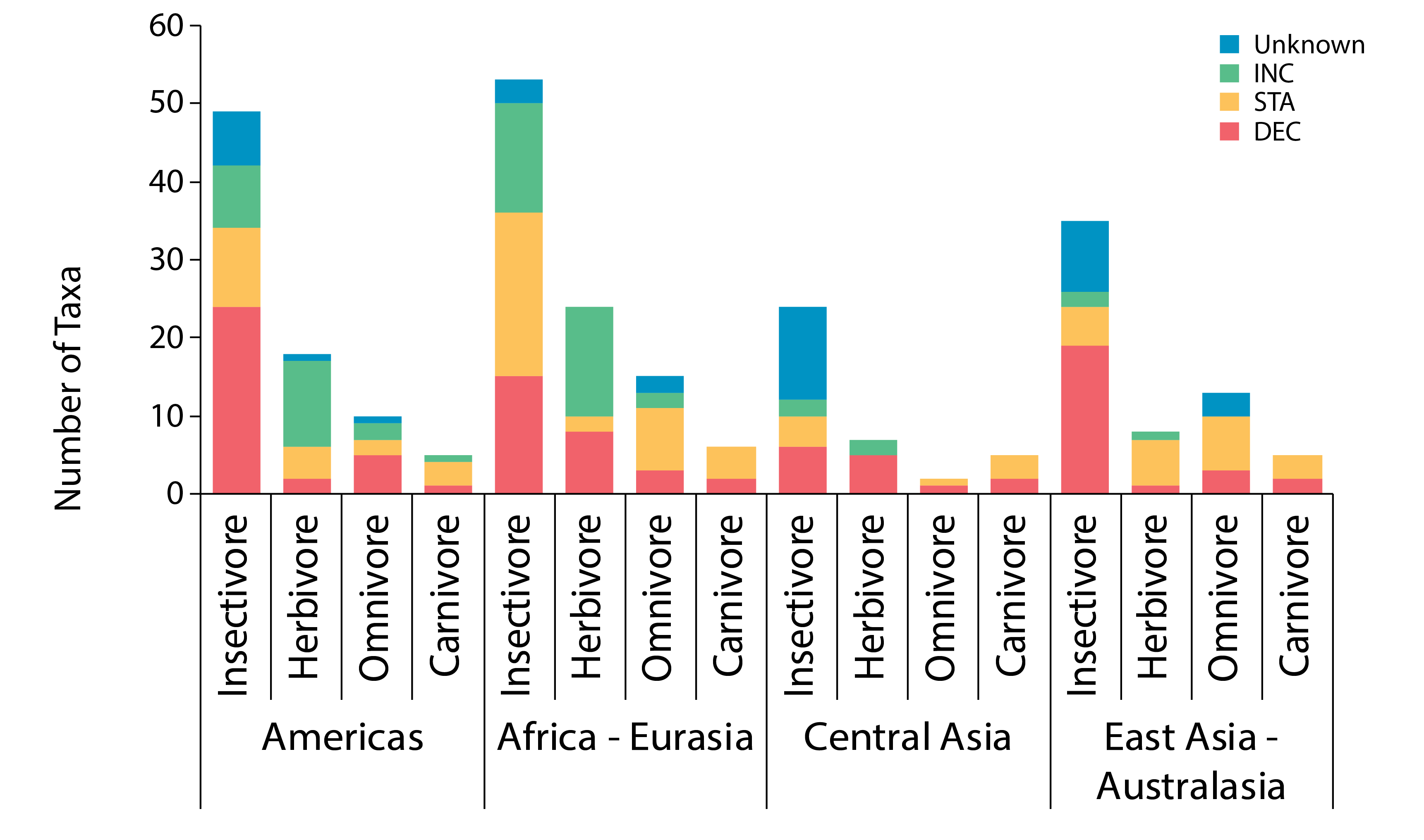
Regional differences are more pronounced in the insectivore guild (Figure 3-24). Although diversity of waders was moderate in the East Asian–Australasian Flyway, 88% (15 of 17) of taxa with known trends were declining—the largest proportion of any group. Both short-term (the last 15 years) and long-term (more than 30 years) trends were available for 157 taxa. Trends were unchanged over the two time periods for 80% of taxa, improved for 11% and worsened for 9%.. STATE OF THE ARCTIC TERRESTRIAL BIODIVERSITY REPORT - Chapter 3 - Page 56 - Figure 3.24
-
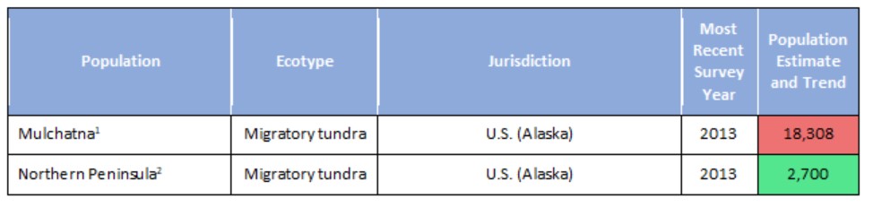
Several smaller populations of caribou inhabit sub-Arctic portions of Alaska, including five populations along the Aleutian Archipelago and west coast. These populations are considered part of the migratory tundra ecotype based on genetics, although in some instances their ecology and habitat are similar to the mountain caribou ecotype found in western Canada. Population dynamics and trends for these populations are variable (Figure 3-29). They are managed by the Alaska Department of Fish and Game through hunting quotas. STATE OF THE ARCTIC TERRESTRIAL BIODIVERSITY REPORT - Chapter 3 - Page 72 - Figure 3.29
-
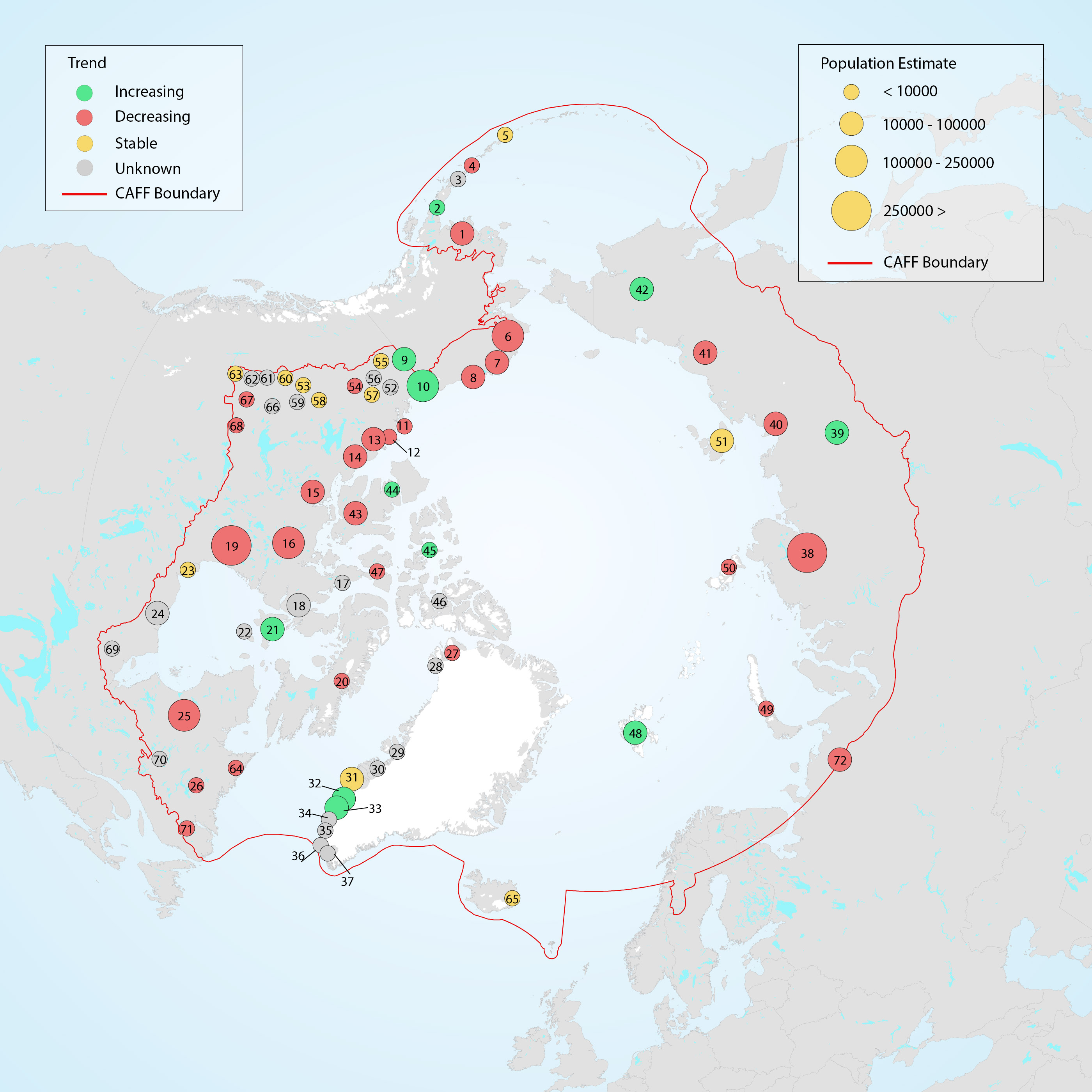
Population estimates and trends for Rangifer populations of the migratory tundra, Arctic island, mountain, and forest ecotypes where their circumpolar distribution intersects the CAFF boundary. Population trends (Increasing, Stable, Decreasing, or Unknown) are indicated by shading. Data sources for each population are indicated as footnotes. STATE OF THE ARCTIC TERRESTRIAL BIODIVERSITY REPORT - Chapter 3 - Page 70 - Table 3.4
-
Many population counts of gregarious migrant species, such as waders and geese, take place along the flyways and at wintering grounds outside the Arctic which stresses the importance of continued development of movement ecology studies. Monitoring of FEC attributes related to breeding success and links to environmental drivers within the Arctic takes place in a wide network of research sites across the Arctic, although with low coverage of the high Arctic zone (Figure 3-25) STATE OF THE ARCTIC TERRESTRIAL BIODIVERSITY REPORT - Chapter 3 - Page 58 - Figure 3.25
-
Temporal trends of arthropod abundance for three habitat types at Zackenberg Research Station, Greenland, 1996–2016. Data are grouped as the FEC ‘arthropod prey for vertebrates’ and separated by habitat type. Solid lines indicate significant regression lines at the p<0.05. Modified from Gillespie et al. 2020a. STATE OF THE ARCTIC TERRESTRIAL BIODIVERSITY REPORT - Chapter 3 - Page 39 - Figure 3.9